B Model Verification
Model evaluation is the process for ensuring that numerical tools are scientifically defensible, transparently developed, and appropriate for use in a given application. Chapter 5 presents a broad examination of NYBEM relative to system quality, technical quality, and usability, which aligns with USACE model certification requirements (EC 1105-2-412). This appendix presents additional analyses undertaken to compare model outcomes (habitat zones and quality) with existing habitat for the region, which we refer to as output verification (McKay et al. 2022). This form of verification generally compares model predictions to independent data sets and includes dozens of methods including not only visual and statistical performance but also correcting for pattern recreation and parameterization issues (Bennett et al. 2013).
The analyses presented in this chapter are an abbreviated version of broader evaluations against empirical data, which are being prepared for peer-reviewed journal articles (Mahan et al. forthcoming; Cordero et al. forthcoming). These analysis are conducted for the existing condition of the New Jersey Back Bays study system. This section includes three main elements. First, model parameterization is described for this study site. Second, the suite of verification methods are described, which are applied to all six habitat types. Third, model verification results are summarized for the six habitat types.
B.1 New Jersey Back Bays (NJBB) Study System
This section presents a preliminary application of the NYBEM to assess ecosystem condition in the New Jersey Back Bays following three main activities: (1) Collection of hydrodynamic model outcomes, (2) Compilation of other environmental input data sets, and (3) Data post-processes and model execution. Additional description of data and models will be included in the NJBB feasibility study’s supplemental EIS.
B.1.1 Hydrodynamic Modeling
NYBEM is capable of reading in hydrodynamic conditions from empirical or modeled data sources. However, hydrodynamic models provide the primary basis for USACE planning because of their capacity to span large spatial domains and forecast outcomes over long time horizons with and without project actions. Adaptive Hydraulics (AdH) is the numerical model code applied for hydrodynamic simulations in this study of the New Jersey Back Bays. The two-dimensional (2D) shallow water module of AdH was applied for all simulations, which solves for depth-averaged velocity and salinity throughout the model domain. (More details of the 2D shallow water module of AdH and its computational philosophy and equations are available in Savant et al. 2014 and Savant and Berger 2015.) AdH version 4.6 was applied for this study.
A 2D AdH model was developed and validated for simulation of hydrodynamics and salinity (Details provided in McAlpin and Ross, draft). The model was validated to available field data for all parameters. Field data were collected in February 2019 for salinity and discharge/velocity data over a 13-hour tidal cycle at three major inlets – Barnegat, Little Egg, and Great Egg. Field data supported the use of a 2D model as opposed to a three-dimensional (3D) model due to lack of major salinity stratification. The model domain was determined using aerial images and bathymetric/topographic data for the area. The Surface Water Modeling System was used to generate a 2D surface mesh and define material regions for applying specific model features, such as bed roughness. The domain is defined horizontally in Universal Transverse Mercator, zone 18 coordinates with units of meters. Vertically it is based on North American Vertical Datum of 1988 (NAVD88) with units of meters. All data applied to the model are shifted to this datum and coordinate system. Bathymetry data for the model were obtained from a variety of sources: the Coastal Relief Model, sponsor collected hydrographic surveys, and the National Elevation Dataset. These data sets were combined such that the latest and highest resolution data were given a larger weighting. The 2D AdH code can include areas that are designated as wet/ or dry; therefore, elevations were included in the domain up to 2 m NAVD88.
The model domain includes over 9,867 square miles, extending approximately 115 miles along the New Jersey Atlantic Ocean coastline from Lewes, DE, to Manasquan, NJ. The 2D mesh contains 324,881 elements and 165,514 nodes. Resolution varies across the domain as needed to capture changes in terrain and features. For instance, fine resolution may be used in small wetland channels to accurately capture the conveyance of flow in these areas as well as the salinity that migrates upstream in deeper channels. Analyses are computed for a one-year simulation with 2018 boundary conditions. For this simulation, the following variables were output:
- Bed elevation
- Water surface elevations: mean lower low water (MLLW), mean tide level (MTL), mean higher high water (MHHW), and 0 to 100% exceedence by 10% (calculated over the 2018 period of record)
- Salinity levels: mean annual and 0 to 100% exceedence by 10% (calculated over the 2018 period of record)
- Velocity: mean annual and 0 to 100% exceedence by 10% (calculated over the 2018 period of record)
AdH outputs were interpolated from point data using a spline technique with barriers separating the marine and estuarine data points (i.e., salinity data were not interpolated over the barrier island) using ESRI Spatial Analyst Tools. The interpolated surfaces were then rasterized throughout the model domain. A 10m grid cell size was used as a balance between data resolution from the model outcomes, over- vs. under-parameterization, and application resolution (i.e., the relevant size of wetlands in the region).
B.1.2 Environmental Data Compilation
Beyond hydrodynamic inputs, other environmental inputs are required for NYBEM.Specifically, these model inputs include, substrate composition, vegetation cover, urban land use composition, shoreline armoring, and vessel traffic.
The estuarine, subtidal model distinguishes hard bottom ecosystems from soft bottom ecosystems (e.g., oysters vs. SAV/clams, respectively). Hard bottom habitats are generally required for reef environments, and this cultch substrate is often a limiting factor in the region. These substrates tend to be less mobile and persist through time. As such, we use a map of historical oyster beds as a proxy for the presence or absence of hard bottom substrate. Shellfish maps from 1963 were digitized that show recreational, moderate commercial, and high commercial uses, all of which were merged into a single hard bottom data layer.
Substrate composition is a major driving factor in both the estuarine and marine subtidal models. Although many nuanced methods exist for assessing substrate (e.g., grain size, distributional metrics, compaction, etc.), simple composition metrics such as percent sand or fine sediment (silt/clay) suffice for the purpose of NYBEM. Furthermore, other substrate metrics are not available at the scale of the NYBEM model domain. Two substrate data sets were combined for this analysis. First, the usSEABED sampling points are available for much of the study area, but underrepresented in the back bay ecosystems. These data were augmented with additional substrate samples from Stockton University and The Nature Conservancy (TNC), which focused explicitly on the NJBB area. Sampling points from these two data sets were combined into a single point cloud and composition metrics were interpolated across the region.
Vegetation cover provides an important and rapid measure of the plant community’s role in ecological function. Cover classes from the NLCD were used to assess this variable. This data set provides cover as a binary (presence / absence) metric at a 30m cell resolution for the entire Nation. A neighborhood analysis was used to translate this binary metric into a continuous variable. Specifically, a moving window assessment was applied with a 50m buffer distance from each raster cell in the NYBEM domain. Vegetation cover percentage was assessed as the mean cover of the cells within this area. The buffer distance of 50m was chosen as large enough to capture multiple cover measurements relative to the grid resolution but small enough to capture the general role of vegetation in the area.
NLCD data were also used to assess the effects of urbanization on estuarine and marine intertidal systems. All urban land uses with the NLCD (codes 21, 22, 23, and 24) were reclassified as urban, and all other types were classified as non-urban. As was the case with vegetation cover, a moving window assessment was applied with a 100m buffer distance from each raster cell in the NYBEM domain. Neighboring urban land use was assessed as the mean cover of the cells within this area. The buffer distance of 100m was chosen to reflect the pervasive influence of urban processes (e.g., noise, light, and water quality) even at relatively large distances from a given patch.
Shoreline armoring also provides an important metric of human use intensity in the intertidal models. The shoreline armoring data layer is a linear dataset developed by the NOAA Office of Response and Restoration. The layer represents linear areas of the coastal shoreline that are armored (i.e., solid man-made structures, riprap, boulder rubble) as of 2014 (NJ) and 2016 (NY). The Environmental Sensitivity Index (ESI) guidelines define these uses for the preparation, evaluation, and/or response to threats to the coastal environment such as oil spills. The shoreline was originally delineated at mean higher high water (MHHW) using Light Detection and Ranging (LiDAR) and high resolution digital orthophotography datasets.
In subtidal and deepwater ecosystems, vessel density provides an important proxy for other human uses like fishing pressure, navigation, and resource extraction. An Automatic Identification Systems (AIS) vessel traffic density raster dataset was generated by the U.S. Coast Guard Navigation Center, Bureau of Ocean Energy Management, and NOAA Office for Coastal Management from AIS Marine Cadastral data. This layer represents 2019 annual vessel transit counts of all vessels (i.e., commercial and recreational) summarized at a 100 m by 100 m pixel cell resolution. A single vessel transit is counted each time a vessel track passes through, starts, or stops within a 100 m grid cell.
B.1.3 Parameter Forecasting
These data sets each represent trade-offs deemed acceptable for this application of the NYBEM. However, different applications could compel use of other data sources. For instance, the NYBEM spatial scale required heavy reliance on regional and national data sets. However, more local applications (e.g., a single bay) could have access to higher resolution data (e.g., locally mapped substrate or shoreline armoring). Data quality and resolution are a common challenge in large scale modeling, and future applications could consider alternative approaches. For this analysis, all data sets were rasterized at the 10m resolution and aligned based on the AdH hydrodynamic data. Table B.1 summarizes all data compilation sources and pre-processing steps. Models were then applied as described in Chapter 4 of this manual.
| Data Layer | Use in NYBEM | Source Data | Post-Processing |
|---|---|---|---|
| Bed elevation (m) | zone | AdH | none |
| Mean lower low water (m) | zone | AdH | none |
| Mean higher high water (m) | zone | AdH | none |
| 10th Percentile Salinity (psu) | zone, est.sub | AdH | none |
| Hard Bottom Substrate (presence/absence) | est.sub | Historic Shellfish Maps | none |
| Intertidal slope | mar.int | AdH | Derived from AdH elevation data |
| Relative exposure time | mar.int | AdH | (Hmax-Hmin) / (MHHW-MLLW) |
| Percent of Light Available | est.sub, mar.sub, mar.deep | AdH | exp(-1.39*Hmedian) |
| Change in Velocity (%) | est.int | AdH | Percent change from 2018 baseline |
| Mean annual salinity (psu) | est.sub | AdH | none |
| Duration of salinity greater than 0.5 psu | fre.tid | AdH | Interpolated from observation percentiles |
| Relative depth | fre.tid, est.int | AdH | (MHWW-Hmed) / (Hmax-Hmin) |
| Median velocity (cm/s) | mar.sub | AdH | Unit conversion from AdH |
| Duration of salinity less than 28 psu | mar.deep | AdH | Interpolated from observation percentiles |
| Neighborhood emergent vegetation cover (%) | fre.tid, est.int, mar.int | NLCD | Percent of cells within 50m having a vegetated class |
| Neighborhood urban land use (%) | est.int, mar.int | NLCD | Percent of cells within 100m having urban land classes |
| Distance to shoreline armoring features (m) | est.in, mar.int | NOAA ESI | Compute distance from centroid of cell to nearest feature |
| Substrate sand composition (%) | est.sub | usSEABED + TNC | Point data merging and interpolation |
| Substrate fines composition (%) | est.sub | usSEABED + TNC | Point data merging and interpolation |
| Vessel Density (tracks per year) | est.sub, mar.sub, mar.deep | AIS | 2019 tracks intersected with raster |
B.2 Methods
NYBEM contains seven sub-models addressing different habitat types (Chapter 4). Three sub-models were verified against independent data sets, specifically: freshwater tidal, estuarine intertidal, and estuarine subtidal. The marine models were not verified due to a lack of a single direct empirical analog data set (e.g., a wetland map), although these models will be verified in the future against multiple data sets (e.g., species distribution observations, water quality metrics).
For each sub-model in the analysis, verification data sets were identified (Table B.2). Specifically, the Coastal Change Analysis Program (CCAP), New Jersey 2012 land use codes (fields, description) and the National Wetland Inventory(fields) served as the primary verification sources. Key attributes or properties of these data sets were extracted for the analysis. All data were aligned with the NYBEM raster mask described above for direct comparison between NYBEM outputs and verification data.
| NYBEM Sub-Model | Verification Data | Attribute or Data Field |
|---|---|---|
| Freshwater Tidal (fresh.tid) | Coastal Change Analysis Program | Palustrine Classes (13, 14, 15, 22) |
| Estuarine Intertidal (est.int) | New Jersey Land Use | saline marsh (6110) and tidal mud flat (5412) |
| Estuarine Intertidal (est.int) | National Wetland Inventory | All estuarine, intertidal systems (E2) |
| Estuarine Subtidal (est.sub) | National Wetland Inventory | Estuarine, subtidal (E1) |
Three families of preliminary analyses were undertaken for each sub-model and verification data set. First, observed habitats were translate into presence and absence outcomes for every grid cell in the NJBB domain (i.e., 1 and 0, respectively). Modeled habitat zones were also translate into presence-absence data for comparison. These data were used to verify the efficacy of NYBEM’s classification methods. For instance, was a given patch correctly or incorrectly categorized as a freshwater tidal ecosystem in the NYBEM relative to a mapped wetland layer? Model results were collected using confusion matrices, which summarize outcomes relative to true positive, false positive, false negative, and true negative classifications. These summary metrics are provided for the entire NJBB domain for each data set.
The second family of verification analyses focused on NYBEM’s habitat suitability predictions. For every patch in a given NYBEM habitat type (e.g., fresh.tid), the overall habitat suitability index (a continuous 0-1 score) was examined relative to presence-absence outcomes from the verification data set. For instance, what was the habitat suitability for all freshwater wetland patches in the verification data set? Ideally, NYBEM would predict high suitability for cells with existing wetlands and low suitability for cells without existing wetlands. Data are summarized for all cells in the NJBB domain with violin diagrams showing the distribution of HSI outcomes relative to presence-absence observations.
The third verification analysis examines the overall predictions of NYBEM at large-scales. The total extent of habitat predicted by NYBEM was summarize in both acreage and habitat units (acreage * habitat suitability) for each of the eleven inlets in the NJBB domain. Ideally, NYBEM would predict the same order-of-magnitude of habitat as observed in each inlet. Data are summarized in plots of observed and modeled estimates of acreage and habitat units.
B.3 Preliminary Results
NYBEM model verification was conducted separately for each sub-model. The following sections summarize verification analyses and discuss the efficacy of the NYBEM as indicated by these outcomes. Notably, model results currently represent an April 2022 version of NYBEM. All modeled outcomes will be updated to reflect this document in September 2022.
B.3.1 Freshwater Tidal Model
The freshwater tidal sub-model was verified against Coastal Change Analysis Program (CCAP) data, specifically the the palustrine classes (codes: 13, 14, 15, 22). Presence-absence outcomes for each cell in the NJBB domain were used to assess the relative rate of classification error. True positive, false positive, false negative, and true negative rates were 1.00%, 8.72%, 9.09%, and 81.21%, respectively. These analyses indicate moderately high rates of misclassification of freshwater tidal habitat.
The freshwater tidal habitat suitability index was examined relative to the presence and absence of CCAP data (Figure B.1). This analysis indicates that NYBEM weakly differentiates habitat quality in patches with and without existing wetlands. Specifically, the mean HSI value for patches with existing wetlands is 0.042 (n=1,179,056), whereas the mean HSI value for patches without existing wetlands is 0.042 (n=10,527,692).
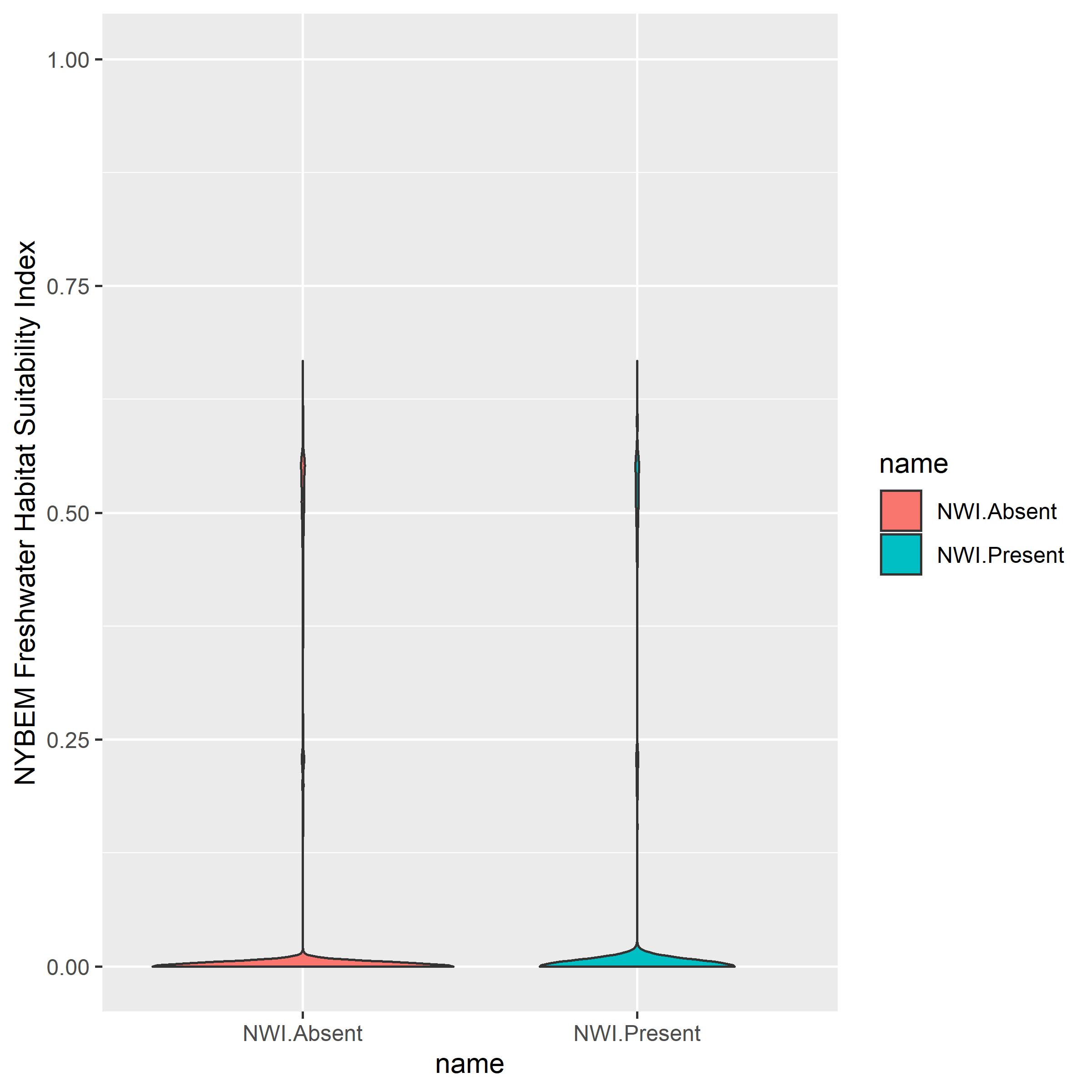
Figure B.1: NYBEM fresh.tid verification relative HSI outcomes in observed CCAP patches.
The final verification analysis examines the aggregate predictions of habitat extent across large-scales. Specifically, the extent of habitat predicted by NYBEM relative to observed habitat on an inlet-by-inlet basis. Figure B.2A shows NYBEM predictions of habitat area only, and Figure B.2B shows habitat quantity and quality via the combined habitat unit. NYBEM delineation criteria are reasonably effective in mapping habitat quantity in the region (Figure B.2A), although NYBEM habitat quality estimates are systematically biased toward significant amounts of under-prediction of wetlands (Figures B.2B). The NYBEM predictions also demonstrate utility in distinguishing the relative amounts of this ecosystem type across inlets, which would indicate utility for assessing relative comparisons with the model (e.g., without and with project conditions).
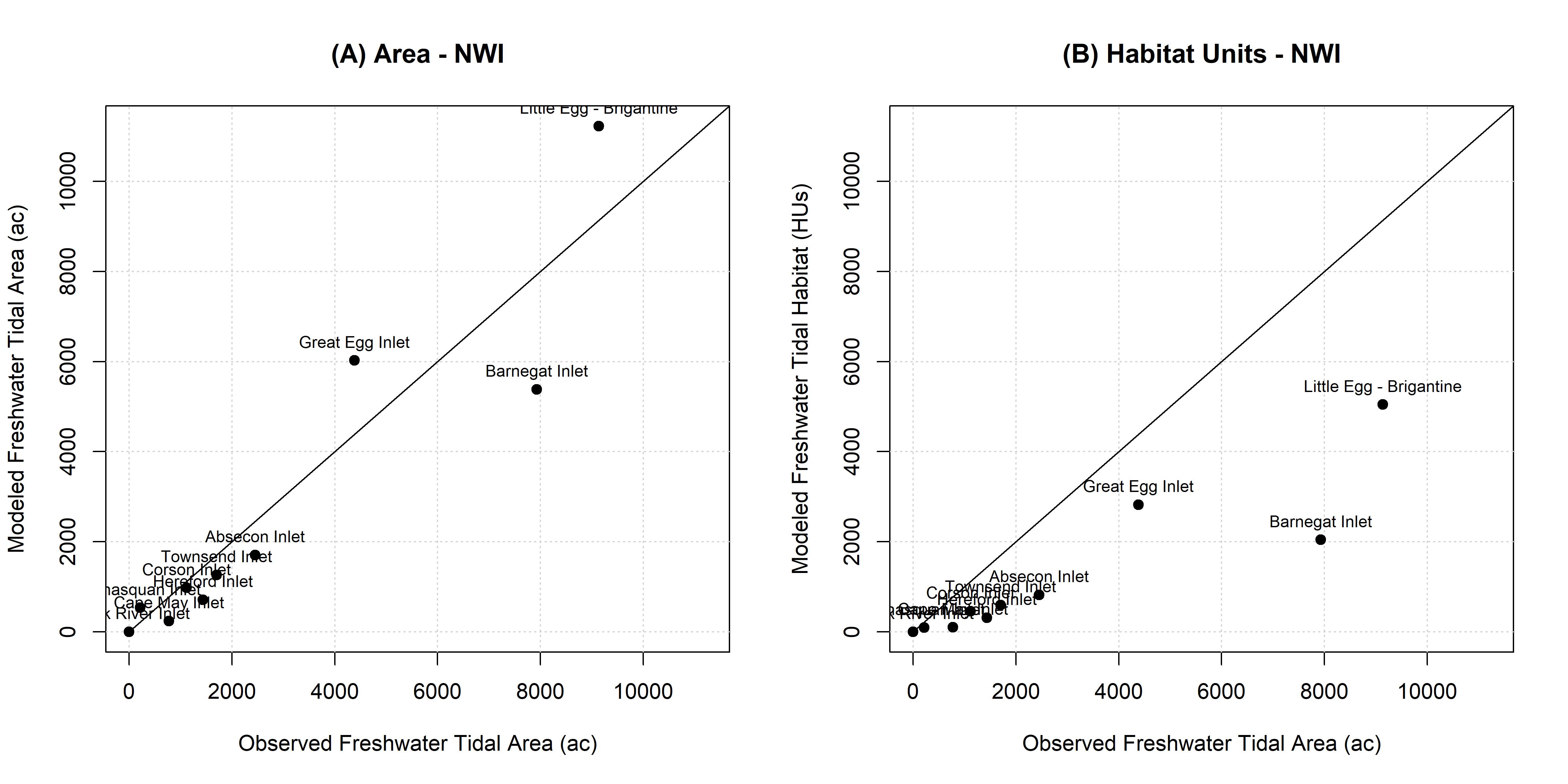
Figure B.2: NYBEM fresh.tid verification relative to the extent of habitat predicted across eleven inlets.
Based on these outcomes, the fresh.tid model has variable utility relative to different outcomes. The habitat quality analysis does not distinguish patches with and without wetlands. However, the delineation criteria provide a useful mechanism for estimating habitat extent. As such, the model should not be used to numerically estimate quality freshwater ecosystems for mitigation purposes. However, the model does strongly differentiate estimates of habitat extent and quality by inlet (Figure B.2), which indicate that relative comparison between systems and alternatives may be appropriate.
B.3.2 Estuarine Intertidal Model
The estuarine intertidal sub-model was verified against the State of New Jersey’s land use classes (codes: 6110 and 5412) and the National Wetland Inventory (code: E2). Presence-absence outcomes for each cell in the NJBB domain were used to assess the relative rate of classification error. For the New Jersey wetlands, true positive, false positive, false negative, and true negative rates were 22.81%, 9.95%, 12.30%, and 54.94%, respectively. For the National Wetland Inventory, true positive, false positive, false negative, and true negative rates were 23.48%, 9.28%, 14.39%, and 52.85%, respectively. These analyses indicate high rates of correct classification (i.e., >75%) and low rates of misclassification (i.e., <25%).
The estuarine intertidal habitat suitability index was examined relative to the presence and absence of the New Jersey and NWI data sets (Figure B.3). This analysis indicates that NYBEM strongly differentiates habitat quality in patches with and without existing wetlands. Specifically, the mean HSI value for NJ wetlands is 0.577 (n=4,108,222), whereas the mean HSI value for patches without existing wetlands is 0.112 (n=7,592,726). The mean HSI value for NWI wetlands is 0.549 (n=4,431,105), whereas the mean HSI value for patches without existing wetlands is 0.109 (n=7,269,846). Figure B.3 also visualizes the misclassification rates discussed above, where false positives appear in the absence data with high HSI (~0.70) and false negatives appear in the presence data with low HSI (~0.0).
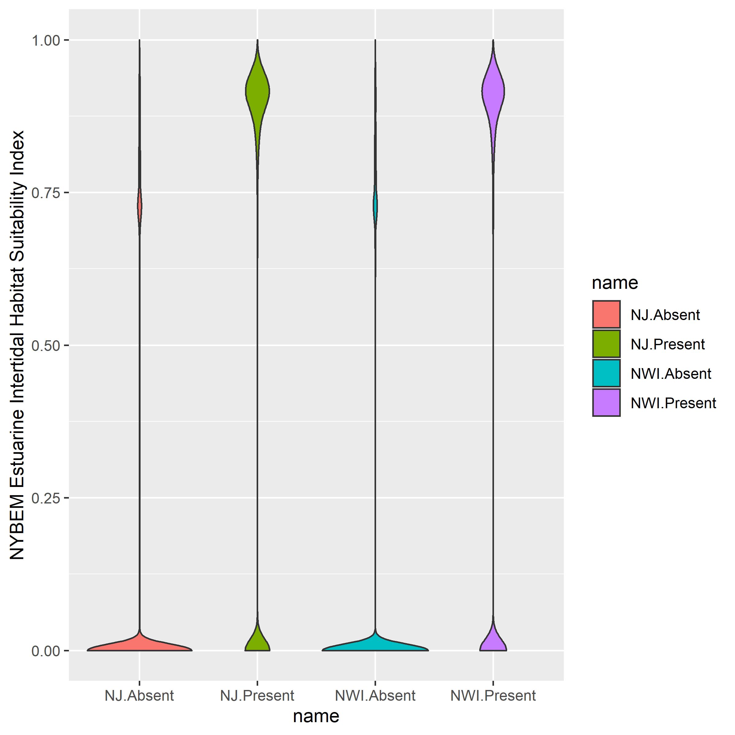
Figure B.3: NYBEM fresh.tid verification relative HSI outcomes in observed NJ and NWI patches.
The aggregate predictions of estuarine intertidal ecosystems across inlets also indicates high model utility (Figure B.4). Total extent of the ecosystem generally aligns well with observed mapping with a bias toward under-prediction (Figures B.4A and B.4C), although some data points deviate significantly (e.g., NYBEM estimates at Barnegat Inlet are lower than NWI observations). NYBEM habitat quality estimates are systematically biased toward under-prediction of wetlands in both the NJ and NWI data (Figures B.4B and B.4D). Notably, the mapped wetlands are not intending to assess quality of given patches. The NYBEM predictions also demonstrate utility in distinguishing the relative amounts of this ecosystem type across inlets, which would indicate strong utility for assessing relative comparisons with the model (e.g., without and with project conditions).
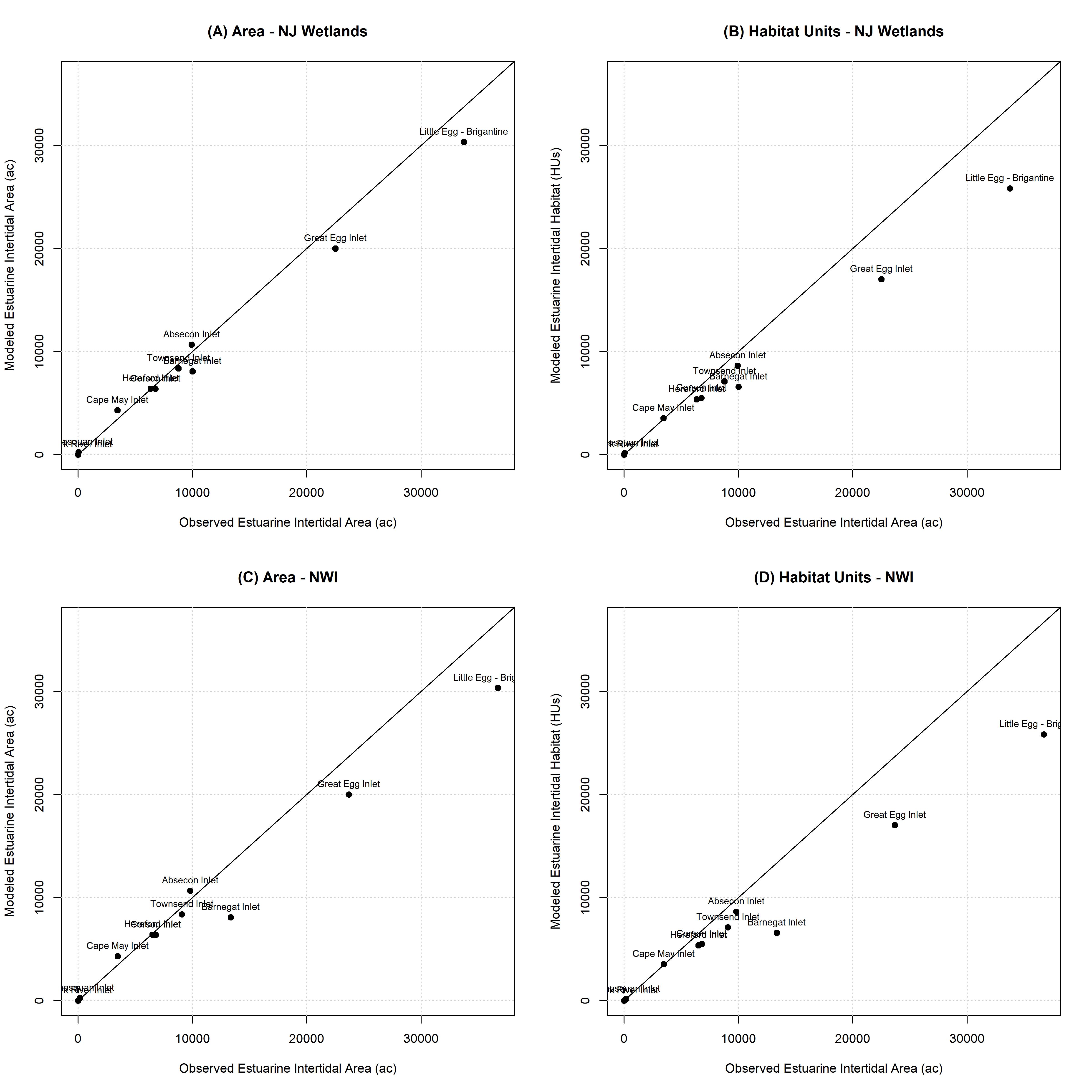
Figure B.4: NYBEM est.int verification relative to the extent of habitat predicted across eleven inlets.
Based on these outcomes, the est.int model reasonably predicts ecosystem extent relative to both binary (i.e., presence-absence) and continuous (i.e., HSI) outcomes. As such, the model could provide a useful framework for estimating a general range of numerical estimates of habitat quantity and quality, and the spread of estimates across inlets indicates high utility for relative comparison between actions at large scales.
B.3.3 Estuarine Subtidal Model
The estuarine subtidal sub-model was verified against the National Wetland Inventory (code: E1). Presence-absence outcomes for each cell in the NJBB domain were used to assess the relative rate of classification error. For the National Wetland Inventory, true positive, false positive, false negative, and true negative rates were 39.57%, 6.05%, 11.15%, and 43.23%, respectively. These analyses indicate high rates of correct classification (i.e., >82%) and low rates of misclassification (i.e., <18%).
The estuarine subtidal habitat suitability index was examined relative to the presence and absence of the NWI data sets (Figure B.5). This analysis indicates that NYBEM strongly differentiates habitat quality in patches with and without existing wetlands. Specifically, the mean HSI value for NWI wetlands is 0.630 (n=5,937,692), whereas the mean HSI value for patches without existing wetlands is 0.108 (n=5,769,056). Figure B.5 also visualizes the misclassification rates discussed above, where false positives appear in the absence data with high HSI (>0.70) and false negatives appear in the presence data with low HSI (~0.0).
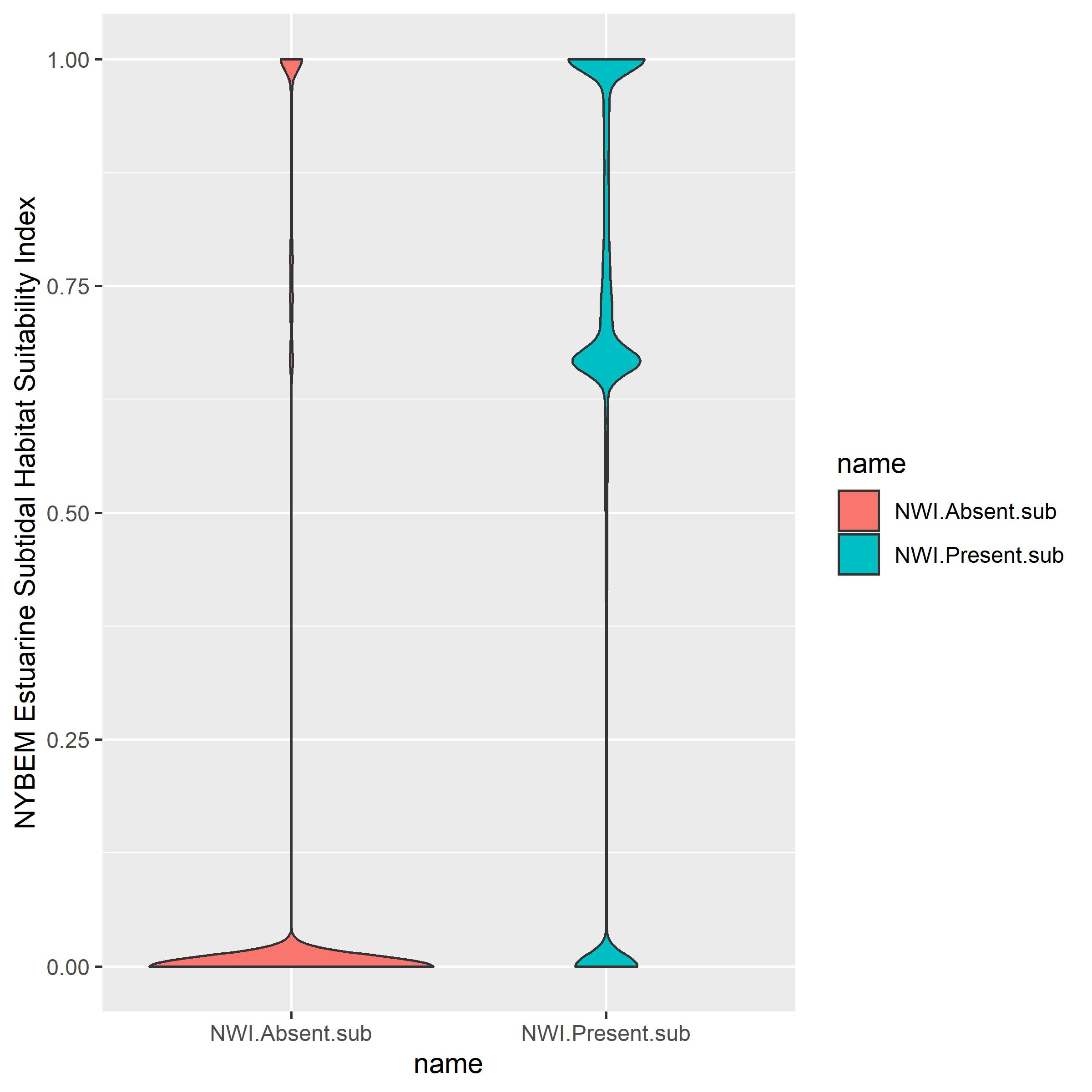
Figure B.5: NYBEM est.sub verification relative HSI outcomes in observed NWI patches.
The aggregate predictions of estuarine subtidal ecosystems across inlets also indicates high model utility (Figure B.6). Total extent of the ecosystem generally aligns well with observed mapping with a bias toward under-prediction (Figure B.6A). NYBEM habitat quality estimates are systematically biased toward under-prediction of wetlands in the NWI data (Figure B.6B). Notably, the mapped NWI wetlands are not intending to assess quality of given patches. The NYBEM predictions also demonstrate utility in distinguishing the relative amounts of this ecosystem type across inlets, which would indicate strong utility for assessing relative comparisons with the model (e.g., without and with project conditions).
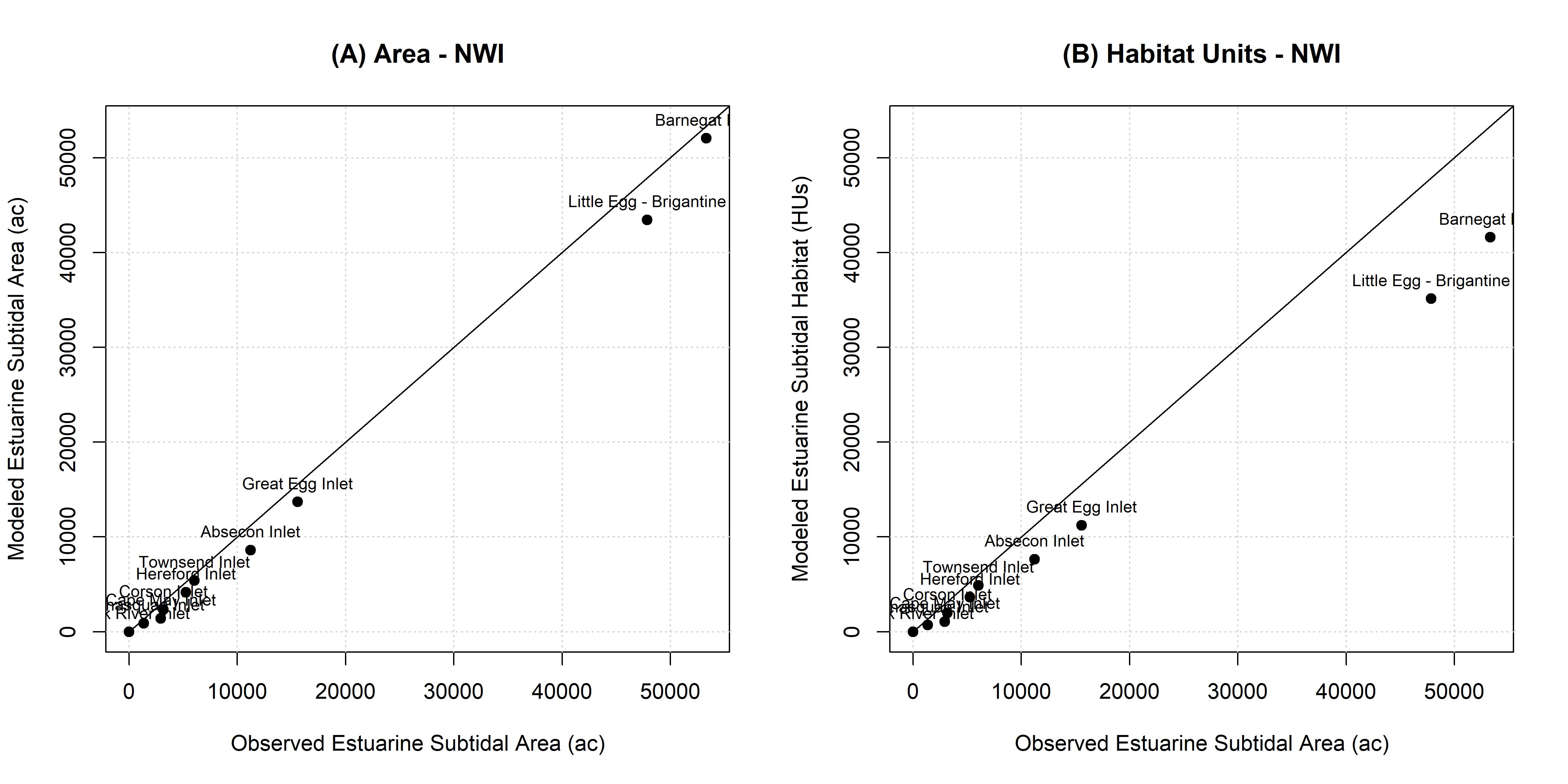
Figure B.6: NYBEM est.sub verification relative to the extent of habitat predicted across eleven inlets.
Based on these outcomes, the est.sub model reasonably predicts ecosystem extent relative to both binary (i.e., presence-absence) and continuous (i.e., HSI) outcomes. As such, the model could provide a useful framework for estimating a general range of numerical estimates of habitat quantity and quality. The spread of estimates across inlets indicates high utility for relative comparison between actions at large scales.
B.4 Summary
The preliminary verification presented here generally lends confidence to the use of NYBEM for relative prediction at large spatial scales. More specifically, the analyses show similar ranges of modeled and observed acreages for the fresh.tid, est.int, and est.sub models. Analyses are underway to better understand patch misclassification error rates.
The est.int and est.sub models also strongly differentiate habitat suitability predictions among sites with and without wetlands. This finding indicates that the models strongly distinguish between features, and the HSI formulation may provide value for distinguishing ecosystem condition. The fresh.tid model does not provide clear differentiation of HSI values, and additional analyses are underway to better understand these effects.
Importantly, the analyses presented here are merely preliminary forms of verification being pursued for NYBEM. First, the marine models were not included in this analysis, and data compilation is underway for validating those models. Second, the approaches used here are somewhat blunt tools in the large spectrum of spatially explicit model validation methods. For instance, more nuanced methods that address issues such as spatial autocorrelation will be pursued as models develop. Third, more sophisticated verification data sets will be used, such as the NWI sub-classes, rather than simply the tidal and salinity criteria. These additional analyses will be published in peer-reviewed journals to vet the utility of the NYBEM framework for large-scale prediction and comparison of ecosystem condition.