Chapter 4 Quantification

The quantification phase of ecological model development formalizes a conceptual model in terms of mathematical relationships, model parameters, and a numerical algorithm (Grant and Swannack 2008). This chapter describes the NYBEM relative to model structure, the theoretical underpinnings of the six ecosystem-specific sub-models, and associated numerical tools. In general, the overarching quantitative architecture of the NYBEM can be summarized in three major elements (Figure 4.1). First, model inputs are assembled in a geospatial database. Second, the model code is prepared as a “package” in the R Statistical Software. Finally, the model outputs habitat quantity and quality as well as habitat units for each patch in the model domain.

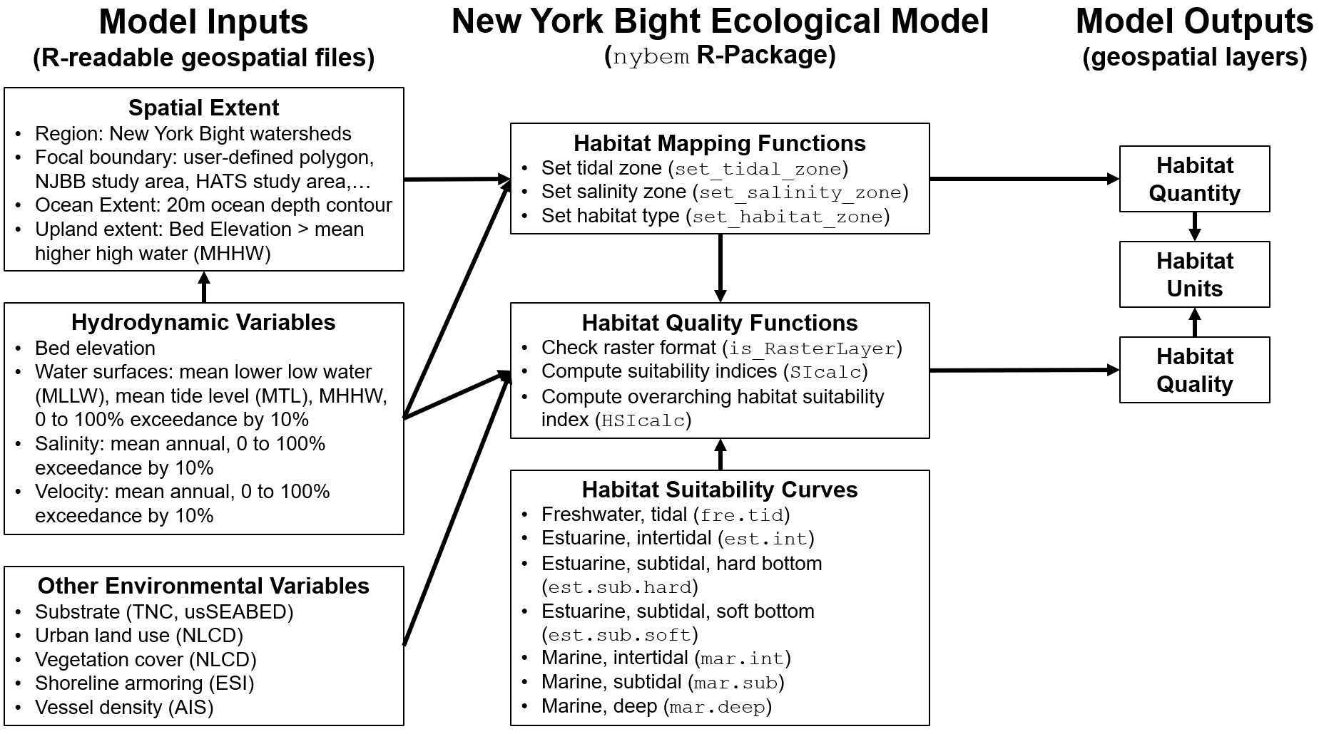
Figure 4.1: Quantitative architecture of the NYBEM.

Variables input into NYBEM consist of three major groups of data layers. First, the spatial extent of a given model run must be defined. The NYBEM is constrained to applications within the region of the New York Bight watersheds (Section 2.1). Within that region, a focal area for the simulation must be specified, which can consist of a particular project boundary (e.g., NJBB or HATS) or a user-specified domain (e.g., a particular back bay). Within that focal area, the downstream and upstream extents of the model are specified based on the 20m ocean depth contour and Mean Higher High Water (MHHW), respectively. The second major group of input variables relate to hydrodynamics. These inputs may be computed over varying temporal windows (e.g., a month, a year, or a decade) depending on the project focus, and the inputs could be provided by a variety of hydrodynamic models or empirical data sources. Hydrodynamic variables characterize the bed elevation, water surface, salinity, and current velocity distributed throughout the project area. Third, a variety of environmental variables are compiled from national and regional data sets to inform habitat quality calculations.

The second major element is the model itself. All model code for the NYBEM is contained within an R-package (nybem, available via github). Generally speaking, a package can be thought of as a fundamental unit of code that can include functions, data, documentation, and tests (Wickham and Bryan 2019). Packages then provide a transportable and reproducible mechanism for code sharing and publication. The nybem package contains three main pieces. Three functions are presented to map the six major habitat types relative to tidal range and salinity. Three more functions contain the computational engine for habitat suitability calculations. Finally, the data for seven different ecosystem-specific suitability models are stored in a list object. Section 4.1 describes the basis for delineating habitat zones, Sections 4.2-4.7 describe the theoretical (i.e., ecological) basis for assessing habitat quality in each zone, and Section 4.8 describes the numerical functions and code in detail.

Each of the habitat quality sub-models followed a consistent set of development steps, which are documented throughout this chapter and briefly described here. Preliminary variables were identified at a series of interagency workshops through a series of conceptual modeling exercises (Appendix A). Additional variables were added based on taxa-specific habitat suitability models (i.e., USFWS “blue books”), relevant tools (e.g., New England Marsh Model), and literature review. A conceptual model was then developed for each ecosystem type to better understand how key variables interact. Regional and national data sets were consulted to ensure that model variables could be assessed throughout the broad spatial extent of the New York Bight, which limited the inclusion of many variables. Potential model variables were compiled along with the rationale for inclusion or exclusion. Finally, a numerical “suitability index” was developed for each variable remaining in the sub-model, which were based on existing suitability indices, published thresholds / responses, and professional judgment. The “suitability indices” should be thought of as generalized metrics of ecosystem condition rather than habitat suitability for a specific taxa. The language of suitability is adopted due to familiarity of decision-makers in the USACE and other environmental management organizations.

The final major element of the modeling framework is the outputs. Ultimately, the nybem package allows users to assess the extent (i.e., quantity) and integrity (i.e., quality) of six major ecosystem types. The size and quality of a given habitat patch can provide useful metrics in their own right, or they may be summarized as an overarching “habitat unit” (i.e., the quantity of habitat in acres * patch quality assessed on a 0 to 1 scale). While nybem outputs these quantities, post-processing is often required outside of the model to interrogate, summarize, and visualize outcomes.

4.1 Habitat Zonation

Throughout this report, the terms “habitat” and “ecosystem” are used synonymously to describe a generally homogeneous classification of an integrated biotic, abiotic, and social system occurring in a given area. Six different ecosystem types are included in NYBEM, and this section describes how these conceptual ecosystems were numerically delineated. The generalized criteria for delineating ecosystems (Table 3.2) were reframed as a suite of logic statements for identifying the salinity zone, tidal zone, or ecosystem type / habitat zone for any given patch.

Tidal zone (\(Z_{tidal}\)) is defined as a categorical metric of deep (1), subtidal (2), intertidal (3), and upland (4) classes.

\[Z_{tidal} = \begin{pmatrix} deep(1) & elev_{bed} < -2m\\ subtidal(2) & -2<elev_{bed}<MLLW\\ intertidal(3) & MLLW<elev_{bed}<MHHW\\ upland(4) & MHHW<elev_{bed} \end{pmatrix}\]

Where \(elev_{bed}\) is bed elevation, \(MLLW\) is mean lower low water, \(MHHW\) is mean higher high water, and all elevations are presented relative to mean tide level.

Salinity zone (\(Z_{salinity}\)) is defined as a categorical metric of marine (1), estuarine (2), and fresh (3) classes.

\[Z_{salinity} = \begin{pmatrix} marine(1) & sal_{10}>28psu\\ estuarine(2) & 28psu>sal_{10}>0.5psu\\ fresh(3) & sal_{10}<0.5psu \end{pmatrix}\]

Where \(sal_{10}\) is a representative low salinity (e.g., average annual low flow, 10th percentile) in practical salinity units (psus).

Habitat zones (\(Z_{habitat}\)) may then be defined from logical combinations of tidal and salinity zones.

\[Z_{habitat} = \begin{pmatrix} upland(1) & Z_{tidal}=4\\ mar.deep(2) & Z_{salinity}=1,Z_{tidal}=1\\ mar.sub(3) & Z_{salinity}=1,Z_{tidal}=2\\ mar.int(4) & Z_{salinity}=1,Z_{tidal}=3\\ est.sub(5) & Z_{salinity}=2,Z_{tidal}=or(1,2)\\ est.int(6) & Z_{salinity}=2,Z_{tidal}=3\\ fresh.tid(7) & Z_{salinity}=3,Z_{tidal}=or(1,2,3) \end{pmatrix}\]

Where \(upland\) represents upland areas outside of the model domain, \(mar.deep\) represents marine, deepwater zones, \(mar.sub\) represents marine, subtidal zones, \(mar.int\) represents marine, intertidal zones, \(est.sub\) represents estuarine, subtidal zones, \(est.int\) represents estuarine, intertidal zones, and \(fresh.tid\) represents freshwater, tidal zones.

4.2 Freshwater, Tidal Zone

Tidal freshwater marshes are found in the topmost region of the estuary where the entry of saltwater from tidal action is mitigated by a significantly higher amount of freshwater from upstream. These unique environments are highly influenced by inflows of freshwater and sediment from rivers. Salt concentrations in tidal freshwater are typically less than 0.5 psu, although larger salinity pulses can occur during spring tides or periods of extremely low river discharge.

Tidal freshwater marshes provide significant nesting sites for a variety of species, including the marsh wren and other organisms dwelling in emergent vegetation. Sea-level rise pushes additional salinity into these systems, causing vegetation to shift and some tidal freshwater marshes to become oligohaline wetlands. Many migratory fish species also rely on this habitat as key resting and stopover areas during migration (Pasternack, Hilgartner, and Brush 2000). Mussels, sturgeon, herring, and marsh wren are some of the taxa of greatest management focus in this ecosystem.

Figure 4.2 presents a conceptual model of the freshwater, tidal ecosystem. In general, this ecosystem can be thought of as strongly driven by marsh elevations and salinity regimes as well as its role as a key transitional habitat between freshwater and saltwater systems. Marsh elevations are governed by interlinked dynamics related to edge erosion, sediment deposition, and organic matter accretion. Salinity regimes are affected by the complex interplay of coastal connectivity and freshwater flows. Migratory processes can be thought of relative to physical barriers affecting pathways (e.g., culverts, tide gates) as well as the value of any given patch for supporting migration via resting and foraging.

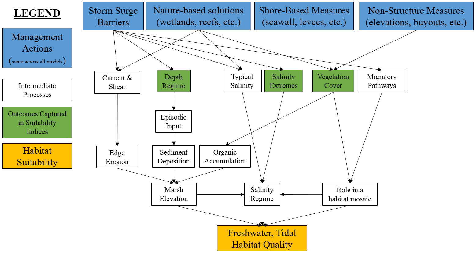
Figure 4.2: Conceptual model for the freshwater, tidal submodel.

Within NYBEM, three general metrics are used to reflect these complex dynamics (Figure 4.3): salinity, vegetation cover, and sediment deposition. Salinity concentration influences many chemical and physical ecological processes within the tidal freshwater ecosystem and supports euryhaline organisms. Emergent vegetation coverage provides habitat, mitigates inland flooding, affects organic matter accretion, and supports water quality within the tidal freshwater ecosystem. Water depth fluctuations support sediment deposition that bring an influx of inorganic sediment and organic nutrients into the ecosystem to mitigate against sea level change. The overall habitat suitability of the freshwater, tidal zone may then be aggregated into a single metric via an arithmetic mean of suitability indices for these three metrics.

\(I_{fresh.tid} = \frac{salinity + veg.cover + deposition}{3}\)

Where \(I_{fresh.tid}\) is an overarching index of ecosystem quality for the freshwater, tidal zone, \(salinity\) is a suitability index relative to salinity, \(veg.cover\) is a suitability index relative to vegetative cover, and \(deposition\) is a suitability index relative to episodic deposition of sediment. All indices are quality metrics scaled from 0 to 1, where 0 is unsuitable and 1 is ideal.

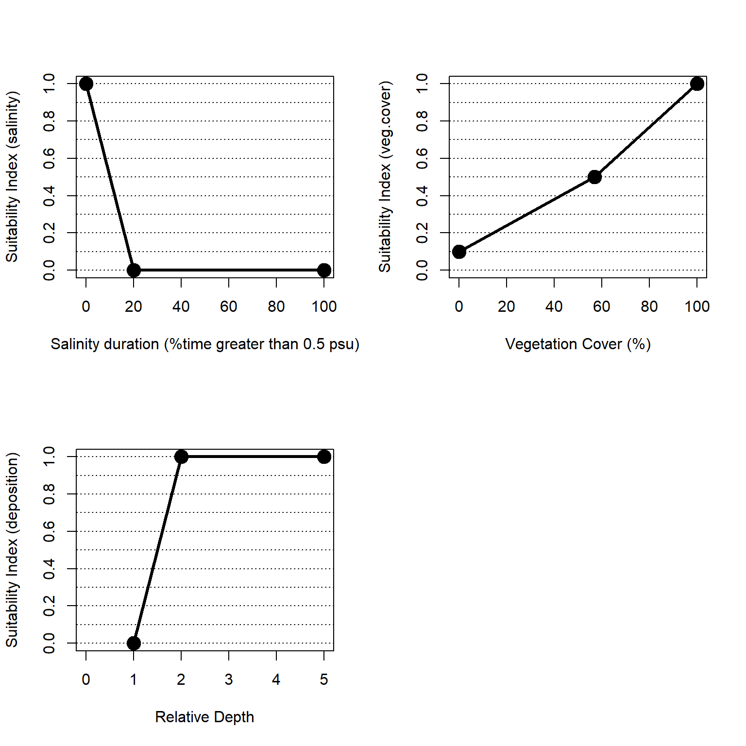
Figure 4.3: Suitability index curves for the freshwater, tidal zone.

4.2.1 Salinity

Freshwater tidal wetlands are regularly flooded marshes and swamps with water that is less saline than brackish. The salinity of the water varies from totally fresh to oligohaline (0 psu to 0.5 psu). Salinity influences physical and chemical processes such as flocculation and the amount of dissolved oxygen (DO) in the water column, as well as the types of organisms that reside in a freshwater tidal ecosystem. Hurricanes and other storms may bring brackish water into the system, which is a significant natural disturbance. Because many plant species in these wetlands are not tolerant to brackish conditions, vegetation can be harmed as a result of these occurrences.

For NYBEM, the salinity regime is summarized through a metric of the percent of time salinity is greater than the freshwater tidal ecosystem threshold of 0.5 psu. These plant communities cannot withstand long periods of increased salinity (over 0.5 ppt). However, this approach assumes that although saltwater inputs serve as disturbance, some amount of saltwater input can stimulate marshes. Salinity may be computed or measured over an annual or multi-annual period. These data may then be summarized as an “exceedence curve” with thresholds from 0-100% in 10% intervals. This exceedence curve may then be used to calculate the percent of time salinity is greater than or equal to 0.5 psu.

This duration metric is then translated into a suitability metric as follows:

\[salinity.high.dur = \begin{pmatrix} 0.05*sal_{dur} & sal_{dur}=0-20\\ 1.0 & sal_{dur}=20-100 \end{pmatrix}\]

Where \(salinity.high.dur\) is a suitability index relative to high salinity periods and \(sal_{dur}\) is the percent of time salinity is greater than the threshold for freshwater tidal habitat (i.e., salinity > 0.5 psu).

4.2.2 Vegetation Cover

Freshwater tidal marshes are characterized by the dominance of herbaceous, shrubby, or emergent aquatic vegetation, with little tree canopy. Emergent vegetation coverage plays a crucial role in the ecosystem. For avian taxa like the marsh wren, reproductive appropriateness may be determined by the relative availability of emergent plants for nesting birds (Gutzwiller and Anderson 1987). Vegetation coverage within a freshwater marsh also provides crucial habitat to a variety of other unique animals and organisms. Further, excessively moist or dry periods can cause additional stress to vegetation leaving the habitat susceptible to a salt intrusion event which can destroy vegetation and make the habitat totally unsuitable.

For the NYBEM tidal freshwater ecosystem submodel, vegetation cover is quantified as the percentage of emergent aquatic vegetation. Emergent aquatic vegetation is a key habitat resource for species found within this ecosystem like marsh wren, and marsh wren are a key indicator species of ecosystem health because they are drawn to ideal wetland conditions. These important avian taxa rarely breed in marshes with less than 57% emergent vegetation (Gutzwiller and Anderson 1987), which is used as a threshold for declines (and increases) in ecosystem condition. However, marshes can continue to provide ecological functions even at low levels of vegetation cover, so ecosystem condition only declines to 0.1 for vegetation cover of 0% (following the example of CWPPRA 2007). The cover metric should be computed relative to a “neighborhood effect” of surrounding patches, which would be indicative of the general condition of the area surrounding the marsh patch.

\[veg.cover = \begin{pmatrix} 0.0070*cover_{per}+0.10 & cover_{per}=0-57\\ 0.0116*cover_{per}-0.16 & cover_{per}=57-100 \end{pmatrix}\]

Where \(veg.cover\) is a suitability index relative to vegetation coverage and \(cover_{per}\) is the percent of vegetation coverage.

4.2.3 Episodic Sediment Deposition

Tidal oscillations control the short-term dynamics of freshwater tidal wetlands, which feed nutrients into the environment and make them more fruitful and productive than some non-tidal wetlands (Propato, Clough, and Polaczyk 2018). These tidal oscillations, as well as irregular weather events, deposit sediment and nutrients into the ecosystem. Increased inundation depths in tidal freshwater marshes can lead to more inorganic sediment deposition, which can assist tidal wetlands keep up with rising sea levels. As a result, marshes can migrate vertically to preserve their position in the tidal frame to some extent.

This metric in NYBEM seeks to capture the benefits of episodic deposition of sediment relative to those of tidal flooding. Episodic sediment deposition requires large magnitude flooding events beyond typical tidal inundation. As such, we developed a metric to assess the relative difference in depth beyond the common tidal datum of MHHW (see equation below). This relative depth metric is one when flood magnitude is equal to MHHW, and the metric increases as flood magnitude increases beyond MHHW. The metric cannot be less than one because the maximum flood is, by definition, greater than a regularly occurring datum.

\[H_{rel} = \frac{H_{max} - H_{median}}{H_{MHHW} - H_{median}}\]

Where \(H_{rel}\) is a relative depth metric assessing the role of episodic floods, \(H_{max}\) is the maximum depth observed over a period of record, \(H_{median}\) is the median depth observed over a period of record, and \(H_{MHHW}\) is the depth at mean higher high water.

The relationship between relative depth and habitat suitability is shown below. We assume that low values of this metric lead to less sediment deposition and are therefore less preferred, and higher values are more ideal. Suitability levels off beyond \[H_{rel}=2.0\] because of a potential for extremely large storms to induce erosion rather than deposit sediment.

\[deposition = \begin{pmatrix} H_{rel}-1.0 & H_{rel}=1-2\\ 1.0 & H_{rel}=2-5 \end{pmatrix}\]

Where \(deposition\) is a suitability index relative to episodic sediment deposition and \(H_{rel}\) is the change in depth in meters.

4.2.4 Potential extension of freshwater, tidal model

Freshwater, tidal ecosystems are complex, dynamic environments, and this NYBEM submodel provides a simple proxy for the relative integrity of these environments. Future improvements to this modeling approach could include the following:

• Organic matter accretion is important in freshwater tidal ecosystem, particularly for marsh adaptation under sea level change (Schile et al. 2014). Accretion is characterized as the accumulation of plant material, including roots and degraded material, from plants growing in the marsh, as well as growth via deposition of suspended particles during floods (Schile et al. 2014). Accretion rates are becoming a more common practice in sea level rise adaptation tools (e.g., (Morris et al. 2002);(Propato, Clough, and Polaczyk 2018)).
  -Edge erosion can also provide a key mechanism of marsh loss in some systems, and this process could be incorporate through hydrodynamic outputs or proxies such as fetch (Morris et al. 2002);(Propato, Clough, and Polaczyk 2018).
  
• Within NYBEM, freshwater tidal areas currently include all depth ranges of freshwater systems (e.g., large rivers, marshes, etc.). An important area of model improvement could arise through a more depth stratified approach to assessing freshwater tidal systems.

4.3 Estuarine, Intertidal Zone

Estuarine environments include marine water that has been diluted by freshwater input to varying degrees (Prosser et al. 2018). Intertidal ecosystems are found between high and low tide, and thus experience varying influences from both upland and aquatic drivers and stressors. The estuarine intertidal ecosystem considers areas with salinity values from 0.5 to 28 psu and elevation from MHHW to MLLW.

Tidal marshes are vegetated intertidal ecosystems found at the land-sea interface that serve as crucial transition zones for marine, freshwater, and terrestrial processes (Colombano et al. 2021). Their location exposes them to a number of environmental factors (e.g., ocean currents, watershed hydrology) and environmental gradients (e.g., salinity)(Lauchlan and Nagelkerken 2020). Figure 4.4 presents a general conceptual model of this system. Generally speaking, the function of these systems is highly related to sediment processes like edge erosion and episodic deposition, long-term shifts in salinity, and the role of these systems as transitional ecotones from fresh-salt water and upland-aquatic.

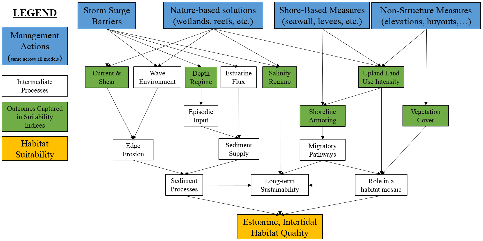
Figure 4.4: Conceptual model for the estuarine, intertidal submodel.

Within NYBEM, five metrics are used to reflect the condition of these systems related to edge erosion, vegetative cover, episodic sediment deposition, development of adjacent uplands, and the presence/absence of shoreline armoring. The overall habitat suitability of the estuarine, intertidal zone may then be aggregated into a single metric via an arithmetic mean of suitability indices for these five metrics.

\(I_{est.int} = \frac{erosion + veg.cover + deposition + upland + shoreline}{5}\)

Where \(I_{est.int}\) is an overarching index of ecosystem quality for the marine intertidal zone, \(erosion\) is a suitability index relative to the edge erosion, \(veg.cover\) is a suitability index relative to vegetative cover, \(deposition\) is a suitability index relative to episodic sediment deposition, \(upland\) is a suitability index relative to adjacent upland land uses, and \(shoreline\) is a suitability index relative to shoreline armoring. All indices are quality metrics scaled from 0 to 1, where 0 is unsuitable and 1 is ideal.

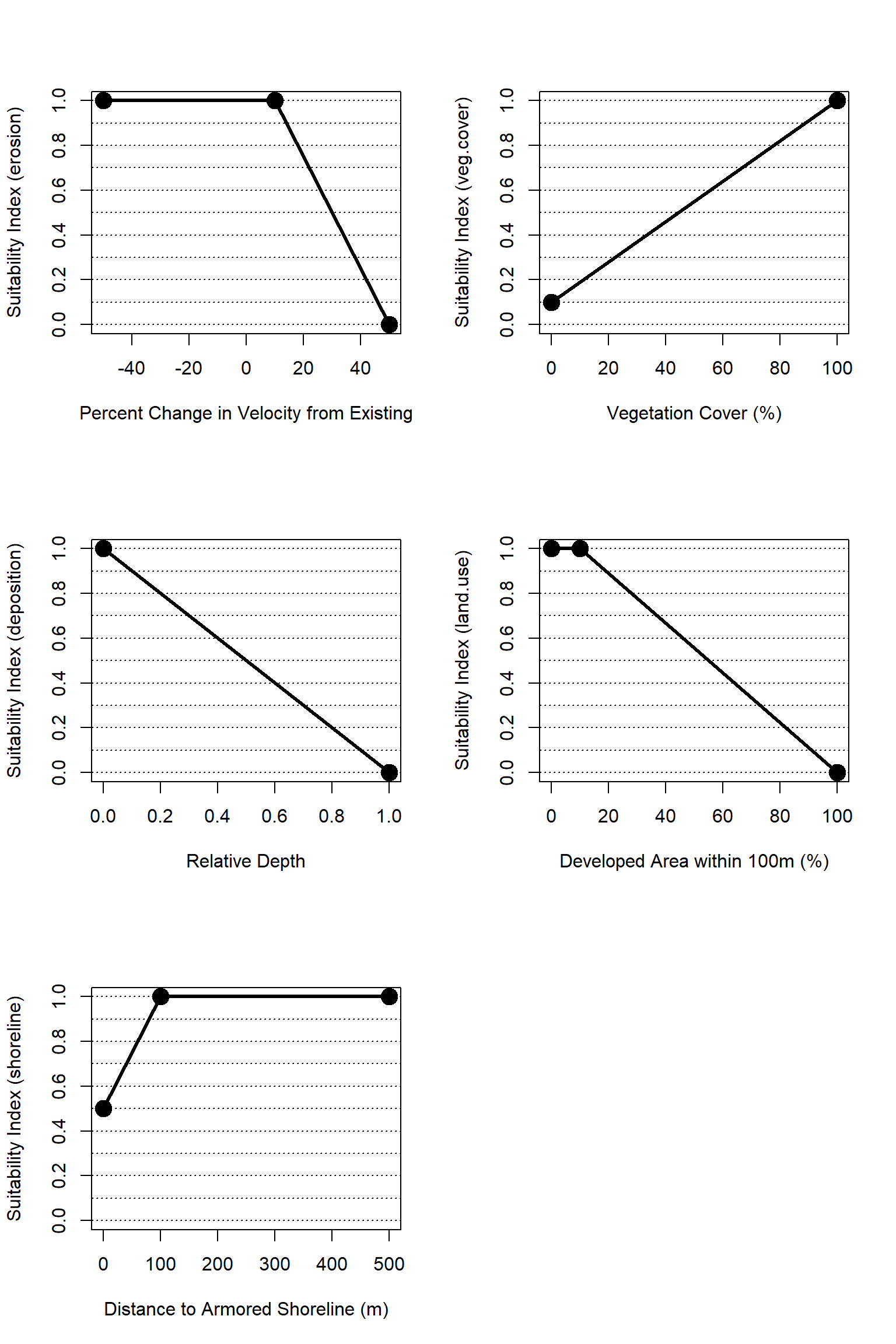
Figure 4.5: Suitability index curves for the estuarine, intertidal zone.

4.3.1 Edge Erosion

Marsh sediment budgets are a geographically integrated measure of opposing constructive and destructive forces: a surplus of sediment can lead to vertical growth and/or lateral expansion, while a shortfall can lead to drowning and/or lateral contraction (Ganju et al. 2017). Many estuarine marshes face sediment deficits along the shoreline as a result of increased edge erosion. Edge degradation causes morphological changes that make it easier for waves to propagate to the marsh borders and promote the resuspension and export of sediments from the estuary (Li, Leonardi, and Plater 2019).

A relative change in velocity from a baseline condition is used as a proxy for more complex edge erosion processes. This assumes that all things being equal, if currents and velocities increase significantly then erosion is likely to increase as well. Notably, increased velocity could result from a future without project condition (e.g., sea level rise), and decrease velocities could result from a future with project condition (e.g., a storm surge barrier). This metric is intended to capture the relative change from current conditions as a proxy for effects of alternative futures on edge erosion rates.

We assume that any increase in high velocity conditions beyond 10% is detrimental, and that increases beyond 50% would fundamentally alter the character of a given marsh. These thresholds were based on input from technical workshops (Appendix A), but the values are largely based on professional judgment and should be reexamined in future models. Importantly, the change in velocity is measured for a high velocity condition, which would generally correlate with storm conditions when erosion would be likely. High velocity conditions are identified as the 90th percentile velocity over a period of record.

\[erosion = \begin{pmatrix} 1.0 & vel_{delta}<10\\ -0.025*vel_{delta}+1.25 & vel_{delta}=10-50\\ 0.0 & vel_{delta}>50 \end{pmatrix}\]

Where \(erosion\) is a suitability index relative to edge erosion and \(vel_{delta}\) is the percent change in high velocity relative to a baseline condition.

4.3.2 Vegetation Cover

Vegetation provides various ecological services within the estuarine intertidal ecosystem, including providing a fish nursery environment, food for migratory birds, nutrient cycling, carbon storage, and sediment stability. The standing density of plant biomass or aboveground production has been demonstrated to result in a positive function in relation to the rate of change of elevation (Morris et al., 2002). Conversely, reductions of vegetative cover can have a significant impact on system functionality. The loss of vegetative cover changes the dynamics in locations that were formerly vegetated. This loss transforms areas of the estuary from a deposition and accretion-friendly environment to one that favors suspension and erosion. For estuaries, high amounts of suspended particles and sediment-associated nutrients create a variety of environmental management issues (Cotton et al. 2006).

For the NYBEM estuarine intertidal submodel, habitat suitability increases as the percentage of vegetative cover increases throughout the habitat. Vegetation cover is quantified as the percentage of emergent aquatic vegetation, and the cover metric should be computed relative to a “neighborhood effect” of surrounding patches, which would be indicative of the general condition of the area surrounding the marsh patch and the marshes long-term sustainability. Marshes can continue to provide ecological functions even at low levels of vegetation cover, so ecosystem condition only declines to 0.1 for vegetation cover of 0% (following the example of CWPPRA 2007).

\[veg.cover = 0.9*cover_{per}+0.1\]

Where \(veg.cover\) is a suitability index relative to vegetation cover and \(cover_{per}\) is the percent of vegetation coverage.

4.3.3 Episodic Sediment Deposition

Estuaries are efficient sediment traps. Marine materials are deposited from the continental shelf into estuarine, littoral habitats. Due to disparities in tidal currents (ebb versus flood tide), sediments are carried to supply sediment on varying time frames. In the estuarine intertidal ecosystem, sediment transport capacity is mostly determined by river discharge, by the timing of discharge events in relation to the spring–neap cycle, and subtidal oscillations in sea level (Prosser et al. 2018).

Periodic flood and storm events are major drivers in sediment dynamics and contribute disproportionately to the total sediment discharge (Ralston et al. 2013). During these episodes of retreating salinity intrusions and increasing bed pressures, sediment deposition episodes can induce considerable bed resuspension in the estuary. The duration of high-discharge episodes in relation to the estuarine reaction time, a feature that fluctuates seasonally with discharge and estuarine length, also affects sediment transport capacity (Palinkas et al. 2014). These short-term events can cause changes in the local biological community and affect seabed stability and strength.

These events then affect sediment mixing and activation which affect water infiltration and exfiltration through the sediment (Nancy Jackson, Karl Nordstorm, and David R. Smith 2010). During storms, erosion of the shoreline can result in the removal of material from the upper foreshore and deposition on the lower foreshore, or the foreshore moving horizontally landward. The influx of additional nutrients following an episode of sediment deposition have been known to cause harmful algal blooms (HABs)(Ralston et al. 2014). Further, the frequent upturn of sediment can displace biological organisms.

The relationship between sediment deposition and water level rise can be used to quantify habitat suitability within the esturarine intertidal ecosystem. When water level increases, sediment deposition will be at an optimal level to support esturarine intertidal habitat. Episodic sediment deposition requires large magnitude flooding events beyond typical tidal inundation. This metric in NYBEM seeks to capture the benefits of episodic deposition of sediment relative to those of tidal flooding. Episodic sediment deposition requires large magnitude flooding events beyond typical tidal inundation. As such, we developed a metric to assess the relative difference in depth beyond the common tidal datum of MHHW (see equation below). This relative depth metric is one when flood magnitude is equal to MHHW, and the metric increases as flood magnitude increases beyond MHHW. The metric cannot be less than one because the maximum flood is, by definition, greater than a regularly occurring datum.

\[H_{rel} = \frac{H_{max} - H_{median}}{H_{MHHW} - H_{median}}\]

Where \(H_{rel}\) is a relative depth metric assessing the role of episodic floods, \(H_{max}\) is the maximum depth observed over a period of record, \(H_{median}\) is the median depth observed over a period of record, and \(H_{MHHW}\) is the depth at mean higher high water.

The relationship between relative depth and habitat suitability is shown below. We assume that low values of this metric lead to less sediment deposition and are therefore less preferred, and higher values are more ideal. Suitability levels off beyond \[H_{rel}=2.0\] because of a potential for extremely large storms to induce erosion rather than deposit sediment.

\[deposition = \begin{pmatrix} H_{rel}-1.0 & H_{rel}=1-2\\ 1.0 & H_{rel}=2-5 \end{pmatrix}\]

Where \(deposition\) is a suitability index relative to episodic sediment deposition and \(H_{rel}\) is the change in depth in meters.

4.3.4 Developement of Adjacent Upland

Land use intensity corresponds to the degree of land transformation caused by technological and economic measures, in addition to urbanization (Ge et al. 2021). Changes in land use intensity can have major impacts on the carbon, nitrogen, and water cycles, and biodiversity and ecological services (Yan et al. 2017). Estuaries serve as a natural buffer between an upland and the coastal areas by filtering urban and agricultural runoff and trapping sediments that can harm aquatic life, absorbing and slowing floodwaters, absorbing wave energy and slowing down currents via wetland plants, all of which prevent erosion and stabilize the shoreline (Ji 2017). A wetland’s value is also greater if it is located near other natural habitats, and that value increases with the degree of connectivity to and complexity of associated habitats (McKinney, Charpentier, and Wigand 2009a).

Furthermore, the development of uplands within a watershed can have a direct and indirect impact on a variety of essential aspects in estuarine intertidal ecosystems. The combination of coastal erosion and upland development causes a “coastal squeeze,” in which low-lying, intertidal regions, that would usually recede inland in the face of sea-level rise, are diminished because man-made structures (e.g. shoreline armoring) prevent such retreat (Prosser et al. 2018). Land management methods on the tidal marsh’s upland border can help or hinder ecosystem migration in response to increasing sea levels (Anisfeld, Cooper, and Kemp 2017).

Heavy pressure from residential development can also alter system salinity and induce a shift in community types (Anthony et al. 2009). Neighboring land use intensity can conservatively be estimated by the relative amount of anthropocentric development pressures within a given buffer from a site. Generally, undeveloped uplands have a positive impact on the resilience of an ecosystem. Inversely, adjacency to developed uplands is correlated with a decrease in ecosystem health associated with a greater degree of fragmentation between systems (Hopkinson et al. 2019), with a decreases in habitat suitability beyond 10% of adjacent uplands developed.

For the NYBEM, habitat suitability is modeled as a function of urban development for adjacent uplands. When the percentage of adjacent urban land uses is greater than 10%, habitat suitability in the estuarine intertidal ecosystem declines. When the development of adjacent upland reaches 100% of the estuarine intertidal ecosystem, the habitat is no longer be considered suitable.

\[land.use = \begin{pmatrix} 1.0 & urban_{per}=0-10\\ -0.011*urban_{per}+1.11 & urban_{per}=10-100 \end{pmatrix}\]

Where \(land.use\) is a suitability index relative to adjacent upland land uses and \(urban_{per}\) is the percent of adjacent upland in developed (i.e., urban) land uses within 100m.

4.3.5 Shoreline Armoring

Natural biological processes and human-induced changes to the estuarine intertidal shoreline boundary are considered as components to a complex ecological system. The mean high-tide line is commonly used to determine shoreline boundaries and extent (Kittinger and Ayers 2010). Shoreline modification called armoring has resulted in a considerable loss of coastal ecosystems from erosion, as well as a reduction in the resilience of these systems to disturbance (Kittinger and Ayers 2010). Shoreline armoring involves placing hardened structures like bulkheads and revetments along the shoreline and as sea levels rise, these structures can prevent coastal marshes from spreading upland over time (Gardner and Johnston 2021).

Armoring is widespread throughout the United States, with extensive armoring found near urban areas (Morley, Toft, and Hanson 2012). Shoreline armoring occupies 50-70% of shorelines along urban coastal areas (Dugan et al. 2018). Increasing shoreline development pressure and predicted sea-level rise suggest that the demand for shoreline armoring will continue to rise and expand throughout the future (Gardner and Johnston 2021). Shoreline armoring is correlated with decreased habitat complexity, and a reduction in connectivity to adjacent habitats (Morley, Toft, and Hanson 2012).

The environmental consequences of armoring are context dependent, relying on characteristics of the environment and armoring structural factors (Dugan et al. 2018). The type of structure placed (e.g., seawalls, bulkheads, revetments, libing shorelines) and its relative placement on the coast profile will influence the biological reactions to armoring.

For the NYBEM, estuarine intertidal habitats that lack shoreline armoring are assumed to have increased habitat suitability. The distance to the nearest armored shoreline is used as a proxy to predict the ability for multiple taxa to use the shoreline as migratory pathways. This metric also serves as a proxy for other forms of anthropogenic pressures (e.g., stormwater input).

\[shoreline = \begin{pmatrix} 0.05*dist_{armor}+0.5 & dist_{armor}=0-100m\\ 1.0 & dist_{armor}>100m \end{pmatrix}\]

Where \(shoreline\) is a suitability index relative to shoreline armoring and \(dist_{armor}\) is the distance to the nearest armored shoreline in meters.

4.3.6 Potential extension of estuarine, intertidal models

Estuarine, intertidal ecosystems are incredibly well-studied environments, and many methods exist for assessing this system. NYBEM combines a few common metrics to obtain a general representation of ecosystem condition. However, future analyses could be expanded to include the following:

• Field-based protocols (e.g., (Bartoldus 1994), [McKinney, Charpentier, and Wigand (2009a), (McKinney, Charpentier, and Wigand 2009b), (Raposa et al. 2016)) are available for this system, and methods could be adapted to incorporate field-style processes into models through remote sensing or proxy variables.
  
• The intertidal zone could be further subdivided to capture differences in tidal flats, low marsh, high marsh, and other subdivisions of this important ecosystem.

4.4 Estuarine, Subtidal Zone

This section presents development of the estuarine, subtidal submodel. Estuarine subtidal habitat was defined as areas with elevations between MLLW and -20m with salinities ranging from 0.5 to 28 psu. This submodel seeks to capture the general condition and trajectory of the estuarine subtidal habitat using three different taxa (oysters, submerged aquatic vegetation/SAV, and clams) as indicators of ecosystem quality, each of which provides critical contributions to the overall quality of the ecosystem. Given this indicator species approach, habitat quality is defined relative to these three taxa’s needs based on existing suitability criteria.

A conceptual model of the estuarine subtidal habitat was developed at a mediated modeling workshop (Appendix A). The conceptual model represented the major components affecting ecosystem quality, and three main categories of drivers were identified: physical (water quality, velocity, sedimentation), anthropogenic (vessel traffic and development stress), and biological (SAV, benthic organisms, fish) with interactions among the categories. Conceptual models were then refined in two key ways (Figure 4.6). First, it was assumed that fish habitat quality would be sufficient if oysters, SAV, and clams habitat needs were met, so this variable was removed. Second, substrate type is a major driver of SAV, oysters, and clams and became a point of stratification within the model. The ecosystem was coarsely divided into hard bottom and soft bottom habitats roughly correlated with oysters and SAV/clams, respectively. The unique characteristics and drivers of these habitats led to splitting the estuarine subtidal sub-model into modules for each of these substrate types.

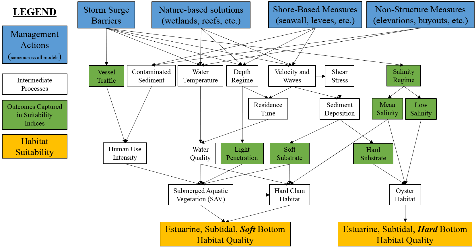
Figure 4.6: Conceptual model for the estuarine, subtidal submodel.

The model was split into hard and soft bottom habitats (est.sub.hard and est.sub.soft, respectively). Hard bottom substrates are crucial for oyster reef establishment and recruitment. Historically, this region had a wide distribution of hard bottom substrate, but anthropogenic influences on water quality, sedimentation, and overfishing have reduced the extent significantly. Here, we use a historical map of oyster reef extent as a proxy for hard bottom with the assumption that hard substrate is relatively immobile and these locations would likely have higher potential for oyster reestablishment. Additional substrates such as gravel, cobble, or ledge provide important habitat and ecological functions, but these habitats were not considered due to a lack of data availability for the large focal area.

4.4.1 Hard Bottom Habitats

Oysters are a major indicator of the integrity of hard bottom habitats in the New York Bight, and the hard bottom submodel is represented by an adaptation of the Oyster Habitat Suitability Index Model (OHSIM, (Swannack, Reif, and Soniat 2014)). The OHSIM is a USACE-certified model for the Eastern oyster (Crassostrea virginica). OHSIM is a spatially-explicit, grid-based index model that uses a series of linear equations to calculate habitat suitability for C. virginica. The model consists of four variables: (1) hard substrate or cultch, (2) mean salinity during spawning season, in which spawning and spat set have a higher optimal salinity than for survival of adults, (3) annual mean salinity, which is the expected range over which adult oysters are viable, and (4) minimum annual salinity, which defines the impacts of high mortality events resulting from lower salinities due to freshwater influxes (Soniat et al. 2012). Variables are briefly described below, and more details can be found in (Swannack, Reif, and Soniat 2014) and USACE model certification reports.

For the NYBEM, spawning season salinity data were not available, so only three variables are used. The overall habitat suitability of the estuarine, subtidal, hard bottom ecosystem is aggregated into a single metric via a geometric mean of these three suitability indices (following the OHSIM).

\(I_{est.sub.hard} = {(cultch * sal.min.ann * sal.mean.ann)}^{1/3}\)

Where \(I_{est.sub.hard}\) is an overarching index of ecosystem quality for the estuarine, subtidal, hard bottom habitats, \(cultch\) is a suitability index relative to hard bottom composition, \(sal.min.ann\) is a suitability index relative to minimum annual salinity, and \(sal.mean.ann\) is a suitability index relative to mean annual salinity. All indices are quality metrics scaled from 0 to 1, where 0 is unsuitable and 1 is ideal.

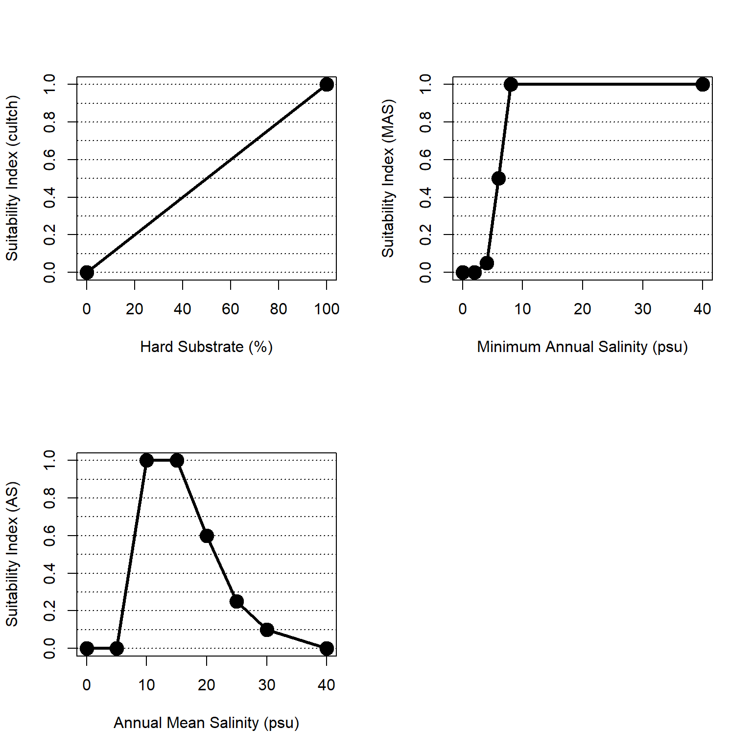
Figure 4.7: Suitability index curves for hard bottom habitats in the esturaine, subtidal zone.

4.4.1.1 Oyster Substrate

Cultch is hard substrate that provides points of attachment and recruitment for spat. Substrate is represented as the percent of the bottom covered with hard substrate, such as existing reefs, or other hard surfaces. We assume that oyster habitat suitability increases linearly from 0 to 100% cultch cover.

\[cultch = 0.01*hard_{per}\]

Where \(cultch\) is a suitability index relative to hard bottom composition and \(hard_{per}\) is the percent of the substrate that is hard bottom.

4.4.1.2 Minimum Annual Salinity

Per Swannack, Reif, and Soniat (2014), Minimum Annual Salinity (MAS) is the minimum value of the 12 monthly mean salinities. This variable is essential to describe freshwater impacts (e.g., freshets, high rainfall years, or freshwater diversions) on oysters and is analogous to the frequency of killing floods variable used by Cake (1983). For NYBEM, we use a representative low salinity (i.e., the tenth percentile, \(sal_{10}\)) rather than a minimum of monthly average. The relationship between MAS and its suitability index is formulated as a linear step-function as follows:

\[sal.min.ann = \begin{pmatrix} 0.0 & MAS=0-2\\ 0.025*MAS-0.05 & MAS=2-4\\ 0.225*MAS-0.85 & MAS=4-6\\ 0.250*MAS-1.00 & MAS=6-8\\ 1.0 & MAS>8 \end{pmatrix}\]

Where \(sal.min.ann\) is a suitability index relative to minimum annual salinity, \(MAS\) is the minimum value of the 12 monthly mean salinities, and \(sal_{10}\) is the tenth percentile of an annual time series of salinity values, a proxy for MAS.

4.4.1.3 Annual Mean Salinity

Annual Mean Salinity (AS) represents the range of salinities over which adult oysters are viable (Cake 1983). The relationship between AS and its suitability index is formulated as a linear step-function as follows:

\[sal.mean.ann = \begin{pmatrix} 0.0 & AS=0-5\\ 0.2*AS-1.00 & AS=5-10\\ 1.00 & AS=10-15\\ 0.08*AS-2.2 & AS=15-20\\ 0.07*AS-2.0 & AS=20-25\\ 0.03*AS-1.0 & AS=25-30\\ 0.01*AS-0.4 & AS=30-40\\ 0.0 & AS>40 \end{pmatrix}\]

Where \(sal.mean.ann\) is a suitability index relative to mean annual salinity and \(AS\) is the mean annual salinity.

4.4.2 Soft Bottom Habitats

Estuarine, subtidal soft bottom habitats comprise large portions of the study areas and host a variety of taxa of interest to environmental management. Specifically, submerged aquatic vegetation (SAV) beds and hard clams are key targets of management. However, these two outcomes have different ecological drivers. As such, the soft bottom model represents a hybridized approach that attempts to assess the general condition of this habitat type relative to both major outcomes.

Habitat suitability is assessed separately for SAV and hard clams. The overall habitat suitability of the estuarine, subtidal, soft bottom ecosystem is aggregated into a single metric via a maximum of the separate suitability indices. This approach assumes that a given patch does not need to be perfect for both taxa simultaneously, but instead, the habitat could have high quality relative to one or the other outcome.

\(I_{est.sub.soft} = max({I_{sav},I_{clam})}\)

Where \(I_{est.sub.soft}\) is an overarching index of ecosystem quality for the estuarine, subtidal, soft bottom habitats, \(I_{sav}\) is a suitability index relative to submerged aquatic vegetation, and \(I_{clam}\) is a suitability index relative to hard clams. All indices are quality metrics scaled from 0 to 1, where 0 is unsuitable and 1 is ideal.

4.4.2.1 Submerged Aquatic Vegetation Module

Submerged aquatic vegetation (SAV) is, generally speaking, a broad grouping of taxa including seagrasses, macroalgae, and other producers, which provide unique habitat structure and ecological function. In NYBEM, a more narrow view of SAV is considered, which focuses broadly on seagrasses and specifically on Zostera marina. The SAV model is represented by three variables critical for growth and reproduction of seagrass, (1) substrate, (2) light availability, and (3) development stress. Suitability scores are represented either as discrete categories or as step functions with linear interpolations between steps.

\(I_{sav} = \frac{substrate.sav + light + vessel.density}{3}\)

Where \(I_{sav}\) is an overarching index of ecosystem quality relative to submerged aquatic vegetation, \(substrate.sav\) is a suitability index relative to fine substrate, \(light\) is a suitability index relative to light penetration, and \(vessel.density\) is a suitability index relative to boat traffic and human uses (a proxy for development stress). All indices are quality metrics scaled from 0 to 1, where 0 is unsuitable and 1 is ideal.

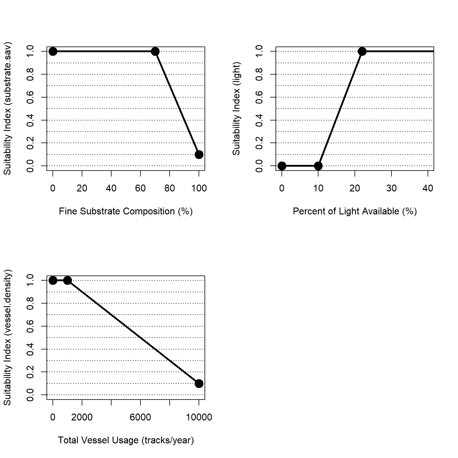
Figure 4.8: Suitability index curves for seagrass in soft bottom habitats in the esturaine, subtidal zone.

Substrate is represented as the presence of soft-bottom sediments conducive for SAV growth. Based on Short et al. (2002), optimal conditions for growth were identified as non-cobble substrates with less than 70% fine sediment. Soft-bottom, non-cobble substrates with greater than 70% fine sediment were considered sub-optimal/adequate. Notably, the suitability index is 0.1 when fines are 100% to indicate the value of fine sediment patches as part of a habitat mosaic (Kritzer et al. 2016). Suitability scores for SAV substrate are represented as follows:

\[substrate.sav = \begin{pmatrix} 1.0 & fines_{per}=0-70\\ -0.030*fines_{per}+3.10 & fines_{per}>70\\ \end{pmatrix}\]

Where \(substrate.sav\) is a suitability index relative to fine substrate and \(fines_{per}\) is the percent of fine substrate (silt and clay).

Light availability drives photosynthesis in SAV. Light attenuates within the water column based on depth and water clarity (i.e., the deeper and more turbid the water, the less light reaches the bottom). For the this model, light availability depends on depth and is calculated algorithmically, then converted into a suitability index. Light availability (\(I_{z}\)) at the plant surface is estimated based on Nes et al. (2003) is calculated as follows:

\[I_{z} = PAR * exp(-K_{d}*z)\]

where \(PAR\) represents the photosynthetically active radiation at the surface, \(K_{d}\) is the light attenuation coefficient for water clarity matching the conditions of the study site, and \(z\) is water depth.

Light attenuation in aquatic systems is a long studied process, although direct measurement of an extinction coefficient (\(K_{d}\)) remains less common. However, Secchi disk depth (\(z_{sd}\)) is a common surrogate for light extinction, and \(K_{d}\) is often estimated (Idso and Gilbert 1974) as:

\[K_{d} = 1.7 / z_{sd}\]

Where \(z_{sd}\) is Secchi depth in meters.

Secchi depth would vary depending on algal productivity, sediment load, water color, and other factors. However, we adopt a regional guideline as a general boundary condition for desirable water clarity. New York State does not have an official standard for Secchi depth, but the state Department of Health requires 1.22 meters (4 feet) of clarity to locate a swimming beach (State 2010). This depth does not represent growth requirements of seagrasses, but it does provide a regionally specific goal for what is perceived as “good” water clarity. This assumption should be revisited in future model applications. This general target aligns with ranges of observations of Secchi depth for the region (McFarland and Hare 2018). Using this standard as a generalized guide for the region, light extinction may be calculated as shown below.

\[K_{d} = 1.7 / 1.22 = 1.39\]

\[PLA = exp(-K_{d}*z) = exp(-1.39 *z)\] Where \(z\) is depth in meters.

Light at the plant surface is converted to a percent of light available (PLA) at that depth, which is used to calculate a suitability score.

\[PLA = \frac{I_{z}}{PAR} * 100\]

The relationship between PLA and its suitability index for SAV is represented as follows. Notably, some studies have indicated a potential saturation effect of light at extremely high PLA (Thayer, Fonseca, and Pendleton 1984); however, light is more likely to be limiting and the suitability curve reflects the more parsimonious situation in which lack of light is a limiting factor.

\[light = \begin{pmatrix} 0.0 & PLA<10\\ 0.0833*PLA-0.83 & 10<PLA<22\\ 1.0 & PLA>22\\ \end{pmatrix}\]

Where \(light\) is a suitability index relative to light penetration and \(PLA\) is percent light available.

Human-mediated disturbances can negatively impact SAV abundance. Many metrics of human disturbance exist quantifying issues like upland urban development, waterway usage, fishing pressures, water quality, and other outcomes. For the purpose of NYBEM, a simple metric of vessel density is used as a proxy for waterway use with the assumption that, all things being equal, a more used waterway is likely to have other anthropogenic pressures (e.g., spills, boat induced waves, etc.). We quantify these disturbances through a proxy of vessel traffic per year. Vessel traffic is obtained from the Automatic Identification System (AIS) database. Thresholds in use were determined by visually inspecting AIS data. Lower traffic (less than 1,000 tracks per year) is considered optimal and the suitability decreases with increasing vessel traffic. Suitability scores for are quantified as follows:

\[vessel.density = \begin{pmatrix} 1.0 & ves_{AIS}=0-1000\\ -0.0001*ves_{AIS}+1.1 & ves_{AIS}=1000-10000\\ 0.1 & ves_{AIS}>10000 \end{pmatrix}\]

Where \(vessel.density\) is a suitability index relative to ship traffic and \(ves_{AIS}\) is the annual vessel tracks over a patch from the Automated Information System.

4.4.2.2 Hard Clam Module

The hard clam habitat suitability submodel is based on an adaptation of Thompson et al. (2021). These authors map hard clam habitat suitability based on salinity, seagrass coverage, flow rates, substrate, cholophyll a, harvesting rates, depth, dissolved oxygen, and temperature. They report ideal depth for hard clams as 4 to 8 m with marginal outcomes in shallower depths, but for this model, depth is assumed to span the entire subtidal range. Only three of the variables recommended by Thompson et al. (2021) were feasible in this analysis: (1) salinity, (2) substrate, and (3) SAV suitability. Data limited the use of all other variables across the large spatial domain of NYBEM. All variables were translated from categorical to continuous suitability scales as follows: optimal (1.0), acceptable (0.75), marginal (0.25), and unsuitable (0.0). The three variables were combined into a single index of ecosystem condition as follows:

\(I_{clam} = \frac{salinity.clam + substrate.clam + sav.prob}{3}\)

Where \(I_{clam}\) is an overarching index of ecosystem quality relative to hard clam habitat, \(salinity.clam\) is a suitability index relative to salinity, \(substrate.clam\) is a suitability index relative to fine substrate, and \(sav.prob\) is an overarching index of ecosystem quality relative to submerged aquatic vegetation coverage. All indices are quality metrics scaled from 0 to 1, where 0 is unsuitable and 1 is ideal.

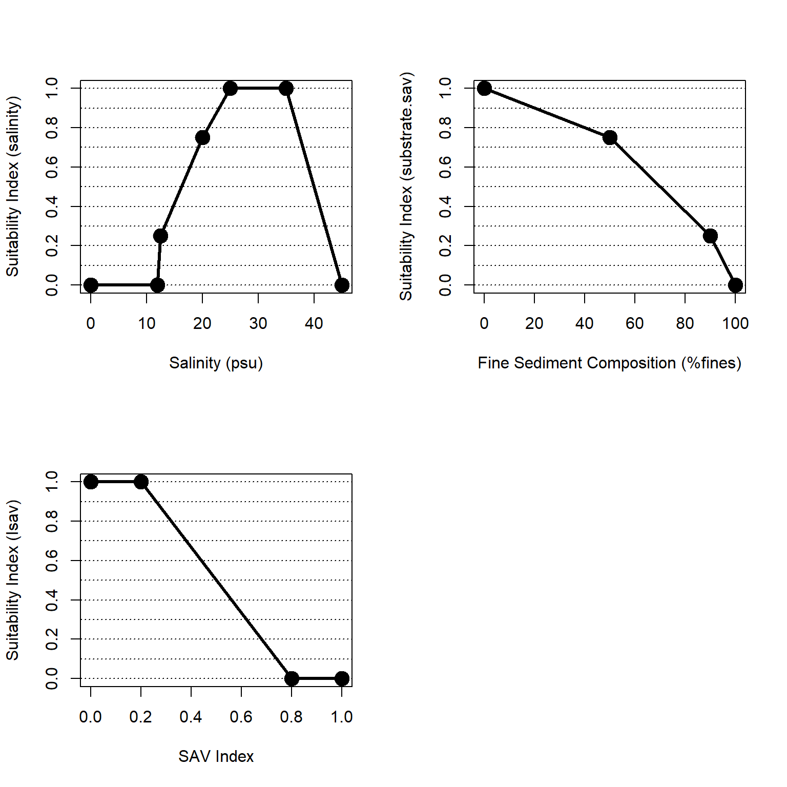
Figure 4.9: Suitability index curves for clams in soft bottom habitats in the esturaine, subtidal zone.

The salinity metric describes the range of salinities over which clams can survive. Optimal salinity for hard clams ranges from 25 to 35 psu. Hyper- and hypo-saline conditions (> 45 or <12.5 psu, respectively) are considered unsuitable when clams are exposed to these conditions for three to six consecutive days. Habitat suitability increases with increasing salinity for intermediate values. The relationship between salinity and its suitability index is formulated as follows:

\[salinity.clam = \begin{pmatrix} 0.0 & MAS=0-12\\ 0.5*MAS-6.0 & MAS=12-12.5\\ 0.033*MAS-0.17 & MAS=12.5-20\\ 0.1*MAS-1.5 & MAS=20-25\\ 1.0 & MAS=25-35\\ -0.1*MAS+4.5 & MAS=12.5-20\\ 0.0 & MAS>45 \end{pmatrix}\]

Where \(salinity.clam\) is a suitability index relative to salinity and \(MAS\) is mean annual salinity.

Similar to seagrass and oysters, substrate is a critical parameter for hard clam viability. Optimal substrate is shelly soft bottom. As the substrate composition increases in fine sediment composition, the substrate becomes less suitable for clams. Suitability scores for clam substrate are quantified as follows:

\[substrate.clam = \begin{pmatrix} 0.0050*fines_{per}+1.00 & fines_{per}=0-50\\ -0.0125*fines_{per}+1.38 & fines_{per}=50-90\\ -0.0250*fines_{per}+2.50 & fines_{per}=90-100 \end{pmatrix}\]

Where \(substrate.clam\) is a suitability index relative to fine substrate and \(fines_{per}\) is fine sediment composition of the substrate (%fines).

Optimal habitat for hard clams is sandy bottom without seagrass. As seagrass coverage increases, the suitability for clams decreases. Given a lack of comprehensive seagrass mapping in the region and an ability to forecast through time, we use the seagrass habitat suitability as a proxy (\(I_{SAV}\)). The relationship between seagrass suitability and hard clam suitability is formulated as follows:

\[sav.prob = \begin{pmatrix} 1.0 & I_{sav}=0-0.2\\ -1.667*I_{sav}+1.33 & I_{sav}=0.2-0.8\\ 0.0 & I_{sav}=0.8-1.0 \end{pmatrix}\]

Where \(sav.prob\) is an overarching index of ecosystem quality relative to submerged aquatic vegetation coverage and \(I_{clam}\) is an overarching index of ecosystem quality relative to submerged aquatic vegetation coverage.

4.4.3 Potential extension of estuarine, subtidal model

As described, the estuarine subtidal ecosystem is a complex environment with multiple ecological outcomes of interest. Any model represents a simplifying set of assumptions, and future modeling could be extended in multiple ways. This submodel makes extensive use of indicator species (i.e., oyster, clam, seagrass), and the use of those taxa and alignment with management objectives should be examined.

The hard bottom model relies on an oyster habitat suitability model, although mean salinity during spawning season was omitted from the NYBEM formulation. This process reflects the higher optimal salinities required for spawning and larval stages (Butler 1954),(Cake 1983) and is an important part of the OHSIM framework, which could be expanded with a more temporally distributed view of processes within NYBEM.

Similarly, the soft bottom model omits some important variables and processes such as:

• Temperature for SAV: Temperature is not presently included but represents a crucial variable for both SAV and clams. Like all vascular plants, temperature is a major driver for SAV viability. At low temperatures, physiological processes are constrained, while metabolic temperature increases with higher temperatures. At temperatures above optimal range for SAV, metabolic activity is significantly reduced or halted as a result of protein denaturation or inactivation (Atkin 2003),(Jensen et al. 2000).

• Temperature for Clams: Water temperature can have significant impacts on hard clams. For future models, temperatures below biological zero (5°C) and above 33°C are likely unsuitable. Temperatures between 12.5°C and above 32°C range in suitability with optimal temperatures between 22.5°C and 30°C.

4.5 Marine, Intertidal Zone

Marine, intertidal ecosystems include the areas of high salinity (> 28 psu) bracketed by tidal limits of the mean higher high water (MHHW) and mean lower low water (MLLW). In the context of NYBEM, these systems tend to directly front the Atlantic Ocean as beaches or occur in high salinity zones near inlets.

Figure 4.10 presents a conceptual model of the marine, intertidal ecosystem. For NYBEM, we focus the assessment of habitat quality primarily on sandy beaches due to the large extent of this habitat type in the region. This nearshore ecosystem is strongly influenced by two major pressures, the physical drivers of the ocean environment (e.g., currents, sediment transport) and human uses of the system (e.g., recreational beach use and associated upland development). Ecologically, this ecosystem hosts a variety of species of management interest such as horseshoe crabs and shorebirds (e.g., piping plover, terns, red knot).

Coastal storm risk management actions have the potential to affect this ecosystem through two primary mechanisms. First, some risk management actions (e.g., storm surge barriers) could be directly constructed in this area. Second, large-scale features have the potential to alter coastal dynamics indirectly, although this affect may occur to a lesser extent given the overarching dominance of ocean effects.

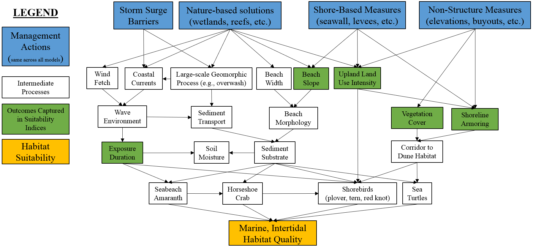
Figure 4.10: Conceptual model for the marine, intertidal submodel.

The tension between human uses of this landscape and ecological outcomes has long been acknowledged, and many models have been developed to assess ecological outcomes in marine, intertidal zones of the region, specifically for sandy beaches. This submodel drew heavily from four general bodies of knowledge, specifically:

• USFWS Habitat Evaluation Procedure models: tern (Carreker 1985), ((USFWS) 2001), Plover ((USFWS) 2001), Horseshoe Crab ((USFWS) 2001), and Red Knot ((USFWS) 2001).
• Other habitat suitability models: Plover Seavey, Gilmer, and McGarigal (2011), Horseshoe Crab (Avissar 2006), (Nancy Jackson, Karl Nordstorm, and David R. Smith 2010), (Lathrope et al. 2013), and amaranth (Sellars and Jolls 2007) (upper intertidal only)
  
• Fire Island to Montauk Point Habitat Evaluation Procedure OceanBeach Sub-Model (USACE 2009).
  
• Empirical studies of the system: Virginia Tech shorebird program (Herman et al. 2019), Rutgers Horseshoe Crab Mapping (Lathrope et al. 2013), and International Shorebird Survey (Manomet).

Four classes of processes and dynamics were identified from a review of these models and studies: long-term and large-scale wave and sediment dynamics, beach morphology, benthic food supplies, and the role of this system as a corridor between aquatic and upland environments. From these processes, four surrogate metrics were identified, which collectively reflect the condition of the marine, intertidal zone. Notably, variables reflecting wave and sediment dynamics are minimally included in this phase of modeling due to assessment challenges. The sections below describe each metric and the rationale in detail, but briefly:

• Beach slope was identified as a proxy for larger effects on overall morphology and grain size.

• The proportion of time a beach is exposed provides a metric of benthic food supplies and availability of foraging habitat.

• Upland land use intensity and shoreline armoring metrics describe the general human use pressures on a given system and viability of corridor functions.

The overall habitat suitability of the marine, intertidal zone may then be aggregated into a single metric via an arithmetic mean of suitability indices for these metrics.

\(I_{mar.int} = \frac{beach.slope + exp.dur + land.use + shoreline}{4}\)

Where \(I_{mar.int}\) is an overarching index of ecosystem quality for the marine intertidal zone, \(beach.slope\) is a suitability index relative to beach slope, \(exp.dur\) is a suitability index relative to the duration of beach exposure, \(land.use\) is a suitability index relative to adjacent upland land uses, and \(shoreline\) is a suitability index relative to shoreline armoring. All indices are quality metrics scaled from 0 to 1, where 0 is unsuitable and 1 is ideal.

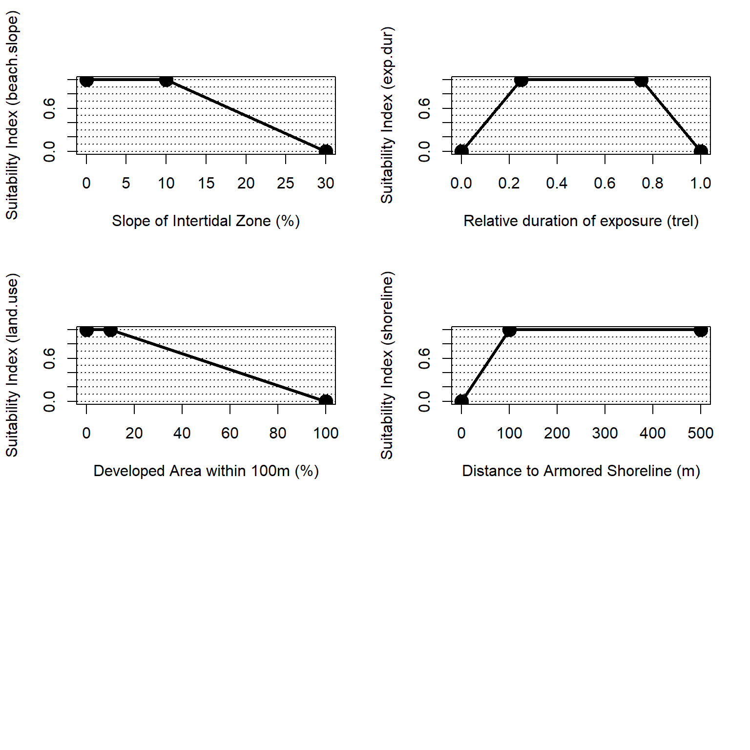
Figure 4.11: Suitability index curves for the marine, intertidal zone.

4.5.1 Beach Slope

Beach morphology directly affects habitat use by multiple focal taxa (e.g., shorebirds, turtles, horseshoe crab). Beach shape and morphologic character can be described through parameters of width, slope, elevation, and other summaries of topography (Bridges et al. 2015). Beach width is indirectly captured in NYBEM through metrics of habitat quantity and patch size and is not considered here. Beach slope integrates morphologic outcomes and is directly tied to grain size and wave environment (Lodder et al. 2021). Beach slope, thus, provides an important and synthetic metric of marine, intertidal habitat quality. Beach slope would only be directly altered for actions in the intertidal zone, but it is included here as a general proxy for intertidal ecosystem condition.

Beach slope is identified as a general indicator of ecosystem condition for Long Island ecosystems (USACE 2009), and as an important driving component of habitat use by multiple taxa in the New York Bight. Specifically, habitat is most suitable for horseshoe crabs between ~5-10% slopes (Brady and Schrading 1996). Notably, not all taxa may respond in kind to these generalization. NYBEM assesses suitability relative to beach slope as follows:

\[beach.slope = \begin{pmatrix} 1.0 & slope_{per}=0-10\\ -0.05*slope_{per}+1.5 & slope_{per}=10-30\\ 0.0 & slope_{per}>30 \end{pmatrix}\]

Where \(beach.slope\) is a suitability index relative to beach slope and \(slope_{per}\) is the slope of the beach perpendicular to the mean tide line in percent.

4.5.2 Exposure Duration

Intertidal zones are a key foraging habitat for shorebirds. The benthic food availability is related in part to soil moisture (Brady and Schrading 1996) and the time to forage in these zones. Soil moisture is also a key determinant of horseshoe crab spawning (Avissar 2006). For instance, in the lower intertidal, we would anticipate higher density of food but less exposure time for foraging; conversely, the higher intertidal would experience lower density of benthic resources but longer exposure time. For NYBEM, a proxy variable is used to account for these processes. Specifically, a ratio of depth ranges to the tidal range is used as a relative duration of exposure, which we calculate as follows:

\[t_{rel} = \frac{H_{max} - H_{min}}{MHHW-MLLW}\]

Where \(t_{rel}\) is a relative duration of exposure, \(H_{max}\) is the maximum depth observed over a hydrodynamic simulation period, \(H_{min}\) is the minimum depth observed over a hydrodynamic simulation period, \(MHHW\) is mean higher high water, and \(MLLW\) is mean lower low water.

This metric provides a relative accounting for the amount of exposure a given path experiences. For instance, \(t_{rel}>1\) occurs in portions of the intertidal that remain underwater most of the time, and \(t_{rel}=0\) occurs in areas where the elevation exceeds the intertidal range. In terms of habitat suitability, we assume that ideal values of this metric occur near the mean tide level (\(0.25<t_{rel}<0.75\)) and suitability declines on either side of this plateau as follows:

\[exp.dur = \begin{pmatrix} 0.04*t_{rel} & t_{rel}<0.25\\ 1.0 & 0.25<t_{rel}<0.75\\ -0.04*t_{rel}+4.0 & t_{rel}>0.75 \end{pmatrix}\]

Where \(exp.dur\) is a suitability index relative to exposure duration.

4.5.3 Upland Land Use

Marine, intertidal zones are a key transitional habitat between aquatic and upland systems. Fully functional intertidal areas would include high-quality adjacent uplands and subtidal areas. A variety of surrogates have been used to assess human impacts on this system, including diverse metrics like foot traffic, vehicle use of beaches, beach grooming and maintenance practices, physical barriers along the beach (Farmer et al. 2000); direct human development such as buildings; trash and debris presence (USACE 2009); and general levels of land use intensity (Seavey, Gilmer, and McGarigal 2011).

For the NYBEM, habitat suitability is modeled based on a relative metric of development for adjacent uplands within 100m. When the percentage of developed adjacent uplands is greater than 10%, habitat suitability in the estuarine intertidal ecosystem declines. When the development of adjacent upland reaches 100% of the estuarine intertidal ecosystem, the habitat will no longer be considered suitable.

\[land.use = \begin{pmatrix} 1.0 & urban_{per}=0-10\\ -0.011*urban_{per}+1.11 & urban_{per}=10-100 \end{pmatrix}\]

Where \(land.use\) is a suitability index relative to adjacent upland land uses and \(urban_{per}\) is the percent of adjacent upland in developed (i.e., urban) land uses within 100m.

4.5.4 Shoreline Armoring

Intertidal areas provide important habitat corridors for organism movement. However, shoreline armoring such as bulkheads or revetments can inhibit movement of the resident taxa (as well as the ecosystem migrating inland with sea level change). Numerous authors have highlighted the negative role that shoreline armoring can play in marine intertidal systems Lathrope et al. (2013). Ideal habitat suitability would occur in the absence of shoreline armoring, but many shorelines are extensively hardened in the developed New York Bight region.

For NYBEM, the distance to the nearest armored shoreline is used as a relative measure of habitat suitability. Habitat is considered more suitable with increasing distance to armoring. NOAA’s Environmental Sensitivity Index (ESI) contains mapped extent of shoreline armoring and is used to assess presence or absence consistently across the region. A suitability index is then assessed as follows:

\[shoreline = \begin{pmatrix} 0.01*dist_{armor} & dist_{armor}=0-100m\\ 1.0 & dist_{armor}>100m \end{pmatrix}\]

Where \(shoreline\) is a suitability index relative to shoreline armoring and \(dist_{armor}\) is the distance to the nearest armored shoreline in meters.

4.5.5 Potential extension of marine, intertidal models

The marine, intertidal model represents trade-offs between habitat needs for multiple taxa and availability of data at regional scales. Future model development could be expanded to include more processes and outcome, specifically:

• A vegetative cover metric may be appropriate for some ecological processes such as the role of this system as a corridor. However, different habitat needs presented a challenge for scoping this metric, and some authors have distinguished the difference in the upper, vegetated intertidal zone and the lower, unvegetated areas (USACE 2009).
  
• Substrate is a key driver of beach outcomes in many contexts (Lodder et al. 2021), and specifically, substrate is often included in regional models of this system (e.g., (Brady and Schrading 1996),(Avissar 2006)). However, high quality substrate data was unavailable, which created a major data gap for incorporating this variable.
  
• Other assessment procedures (Farmer et al. 2000), (USACE 2009) have included a variety of human development pressures related to local features (e.g., vehicle and foot traffic), which could provide important refinement of the human use intensity metrics for land use and shoreline development.
  
• Wave environments clearly affect the morphology of beaches, and additional hydrodynamic variables could be assessed in future models.

4.6 Marine, Subtidal Zone

Marine, subtidal ecosystems include the areas of high salinity (> 28 psu) bracketed by tidal limits of the mean lower low water (MLLW) and 2m below Mean Tide Level (MTL). In the context of NYBEM, these systems tend to directly front the Atlantic Ocean or occur in high salinity zones near inlets.

Figure 4.12 presents a conceptual model of the marine, subtidal ecosystem. This nearshore ecosystem hosts a variety of species of management interest such as hard clams, winter flounder, and seagrasses. As such, this model generally centers on the pelagic systems, submerged aquatic vegetation, and the benthic system. In general, coastal storm risk management actions are more likely to have direct effects on this ecosystem (e.g., footprint of constructed storm surge barriers) than indirect, offsite concerns more common in the estuarine systems.

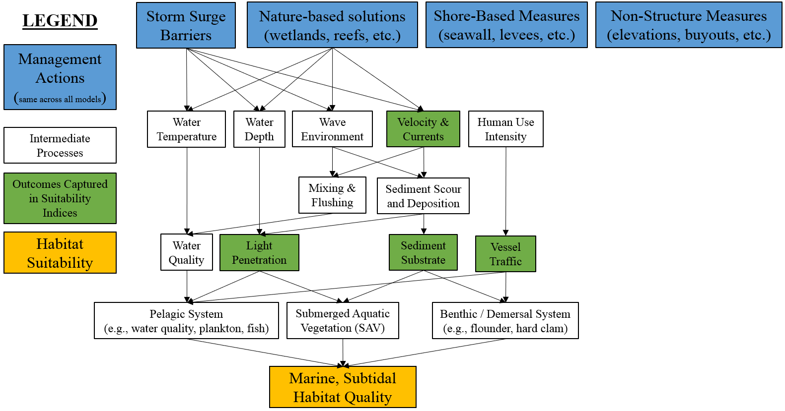
Figure 4.12: Conceptual model for the marine, subtidal submodel.

The tension between human uses of this landscape and ecological outcomes has long been acknowledged, and many models have been developed to assess ecological outcomes in marine, subtidal zones of the region. This submodel drew heavily from three primary bodies of knowledge, specifically:

• NY/NJ harbor mitigation functional assessment models (USACE 2000)

• Habitat suitability models for winter flounder (Banner and Schaller 2001) and hard clam (Mulholland 1984).

• Regional monitoring data associated with NY/NJ Harbor Deepening (USACE 2012), (USACE, n.d.a), (USACE, n.d.b), essential fish habitat mapping (USACE 2013), and water quality data for the lower bay (DEP 2018, (USACE, n.d.b)).

Four main classes of processes and dynamics were identified from a review of these models and studies: (1) substrate-driven habitat use, (2) physical currents and mixing, (3) light penetration, and (4) human uses of the system. For each process, surrogate metrics were identified, which collectively reflect the condition of the marine, subtidal zone. The sections below describe each metric and the rationale in detail, but briefly:

• Current velocity is a major driver of sediment dynamics as well as water quality processes.

• Fine substrate affects utilization of habitats by a variety of taxa.

• Light penetration is a proxy for both water quality outcomes and potential SAV growth.

• Vessel traffic density is a proxy for human use intensity.

The overall habitat suitability of the marine, subtidal zone may then be aggregated into a single metric via an arithmetic mean of suitability indices for these four metrics.

\(I_{mar.sub} = \frac{velocity + substrate + light + vessel.density}{4}\)

Where \(I_{mar.sub}\) is an overarching index of ecosystem quality for the marine subtidal zone, \(velocity\) is a suitability index relative to beach slope, \(substrate\) is a suitability index relative to fine substrate, \(light\) is a suitability index relative to light penetration, and \(vessel.density\) is a suitability index relative to boat traffic and human uses. All indices are quality metrics scaled from 0 to 1, where 0 is unsuitable and 1 is ideal.

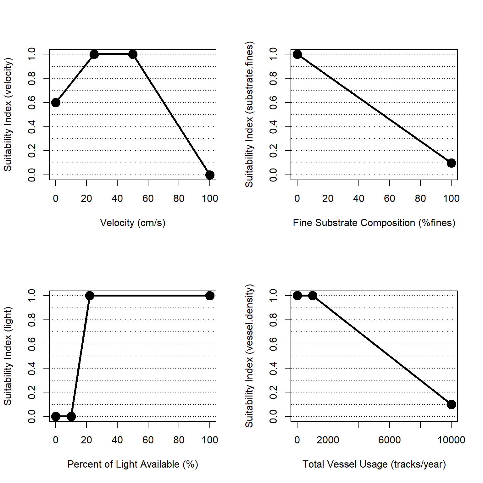
Figure 4.13: Suitability index curves for the marine, deepwater zone.

4.6.1 Velocity

Velocity, currents, and wave environment are a key determinant of habitat suitability as well as critical drivers of sediment dynamics and water quality processes. For example, hard clam habitat suitability is generally in low to moderate velocity environments (<50 cm/s) with declines in suitability up to 100 cm/s. For NYBEM, the velocity suitability for hard clams is adopted directly from Mulholland (1984) as shown below. We assess velocity as the median velocity observed over an annual hydrodynamic simulation.

\[velocity = \begin{pmatrix} 0.016*V_{50}+0.6 & V_{50}=0-1\\ 1.0 & V_{50}=1-10\\ -0.02*ves_{AIS}+2 & V_{50}=10-100\\ 0.0 & V_{50}>100 \end{pmatrix}\]

Where \(velocity\) is a suitability index relative to currents and velocity and \(ves_{AIS}\) is the vessel density from the Automated Information System.

4.6.2 Substrate

Sediment quality drives multiple aspects of ecosystem integrity such as benthic habitat provision, nutrient dynamics, and erodibility. Fine sediment composition (i.e., %fine) is a common metric in multiple assessment procedures in the region (e.g., (Mulholland 1984), (USACE 2000), (USACE 2021)). Specifically, the suitability curve from the hard clam model (Mulholland 1984) is used as the basis for this rapid metric of ecosystem quality. Notably, the curve was modified such that the suitability index is 0.1 when fines are 100%; this change was made in response to more recent literature showing the value of fine sediment patches as part of a habitat mosaic (Kritzer et al. 2016). For marine environments, sediment data are obtained from the usSEABED data set throughout the region. Habitat suitability is then quantified as follows:

\[substrate = -0.009*fines_{per}+1\]

Where \(substrate\) is a suitability index relative to sediment substrate and \(fines_{per}\) is the proportion of fine sediment (silt and clay) at the location.

4.6.3 Light

Light penetration provides an important metric of general water quality as well as suitability for submerged aquatic vegetation. Specifically, light availability drives photosynthesis in SAV. Light attenuates within the water column based on depth and water clarity (i.e., the deeper and more turbid the water, the less light reaches the bottom). For the marine subtidal submodel, light availability and suitability are modeled following the same algorithms described for the estuarine subtidal model (See Section 4.4.2.1), which can be summarized in suitability terms as as:

\[light = \begin{pmatrix} 0.0 & PLA<10\\ 0.0833*PLA-0.83 & PLA>70\\ 1.0 & PLA>22\\ \end{pmatrix}\]

Where \(light\) is a suitability index relative to light penetration and \(PLA\) is percent light available (PLA).

4.6.4 Vessel Density

Human-mediated disturbances (e.g., urban development, increased vessel traffic, etc.) can negatively impact SAV abundance. We quantify these disturbances through a proxy of vessel traffic per year. Vessel traffic is obtained from the Automatic Identification System (AIS) database. Lower traffic (less than 1,000 tracks per year) is considered optimal and the suitability decreases with increasing vessel traffic. Suitability scores for are quantified as follows:

\[vessel.density = \begin{pmatrix} 1.0 & ves_{AIS}=0-1000\\ -0.0001*ves_{AIS}+1.1 & ves_{AIS}=1000-10000\\ 0.1 & ves_{AIS}>10000 \end{pmatrix}\]

Where \(vessel.density\) is a suitability index relative to ship traffic and \(ves_{AIS}\) is the annual vessel tracks over a patch from the Automated Information System.

4.6.5 Potential extension of marine, subtidal model

NYBEM’s marine subtidal submodel provides a simple framework for estimating general ecosystem condition, which was centered on indicator species of hard clam and seagrasses. Other indicator taxa, variables, and processes should be addressed in future iterations where possible. Specifically, substrate is a dynamic feature through time, particularly with sea level change, and substrate could be linked to sediment transport algorithms in coastal dynamics models. Similarly, wave environment is an important feature of this ecosystem, and additional wave metrics could be incorporated. In the present iteration of NYBEM, light attenuation is assumed to be dependent on a single light coefficient (\(K_{d}\)). However, light attenuation can vary significantly based on suspended sediment concentration, algal processes, or water color, all of which may vary in time. Future version of the model could also consider spatially distributed data sets of light coefficients such as those by NOAA.

4.7 Marine, Deepwater Zone

The marine, deepwater ecosystem considers areas with salinity values greater or equal to 28 psu and depths from 2 to 20 m. Physical, biological and chemical variables may be compounded by anthropogenic and climatic pressures to influence the overall integrity of this system. Figure 4.14 presents a conceptual model of the marine, deepwater ecosystem, which is strongly dominated by large-scale oceanographic processes and less so by potential coastal storm risk management features. Ecologically, this ecosystem hosts a variety of species of management interest such as mammals, turtles, surf clams, migratory fish, and flounder (winter).

Figure 4.14: Conceptual model for the marine, deepwater submodel.

The following variables are used to assess the marine deepwater submodel: (1) salinity, (2) velocity and currents, (3) light attenuation, and (4) vessel traffic. Salinity acts as a proxy for vertical mixing of the water column and influence of freshwater inputs (Smit et al. 2021). Current velocities represent mixing and flushing of the system, sediment suspension, and benthic scouring. Light penetration depths within the water column indicate water column turbidity, nutrient loading and algal production levels. Finally, vessel traffic provides an index for development pressures for both commercial and recreational fishing pressure on the pelagic, demersal and benthic systems and commercial and recreational vessel density pressures on the marine mammal populations within the area (population stress from ship strikes and noise). The overall habitat suitability of the marine, deepwater zone may then be aggregated into a single metric via an arithmetic mean of suitability indices for these four metrics.

\(I_{mar.deep} = \frac{salinity.low.dur + velocity.low.change + light + vessel.density}{4}\)

Where \(I_{mar.deep}\) is an overarching index of ecosystem quality for the marine intertidal zone, \(salinity.low.dur\) is a suitability index relative to low salinity periods, \(velocity.low.change\) is a suitability index relative to changes in low velocity, \(light\) is a suitability index relative to light penetration through water, and \(vessel.density\) is a suitability index relative to ship traffic. All indices are quality metrics scaled from 0 to 1, where 0 is unsuitable and 1 is ideal.

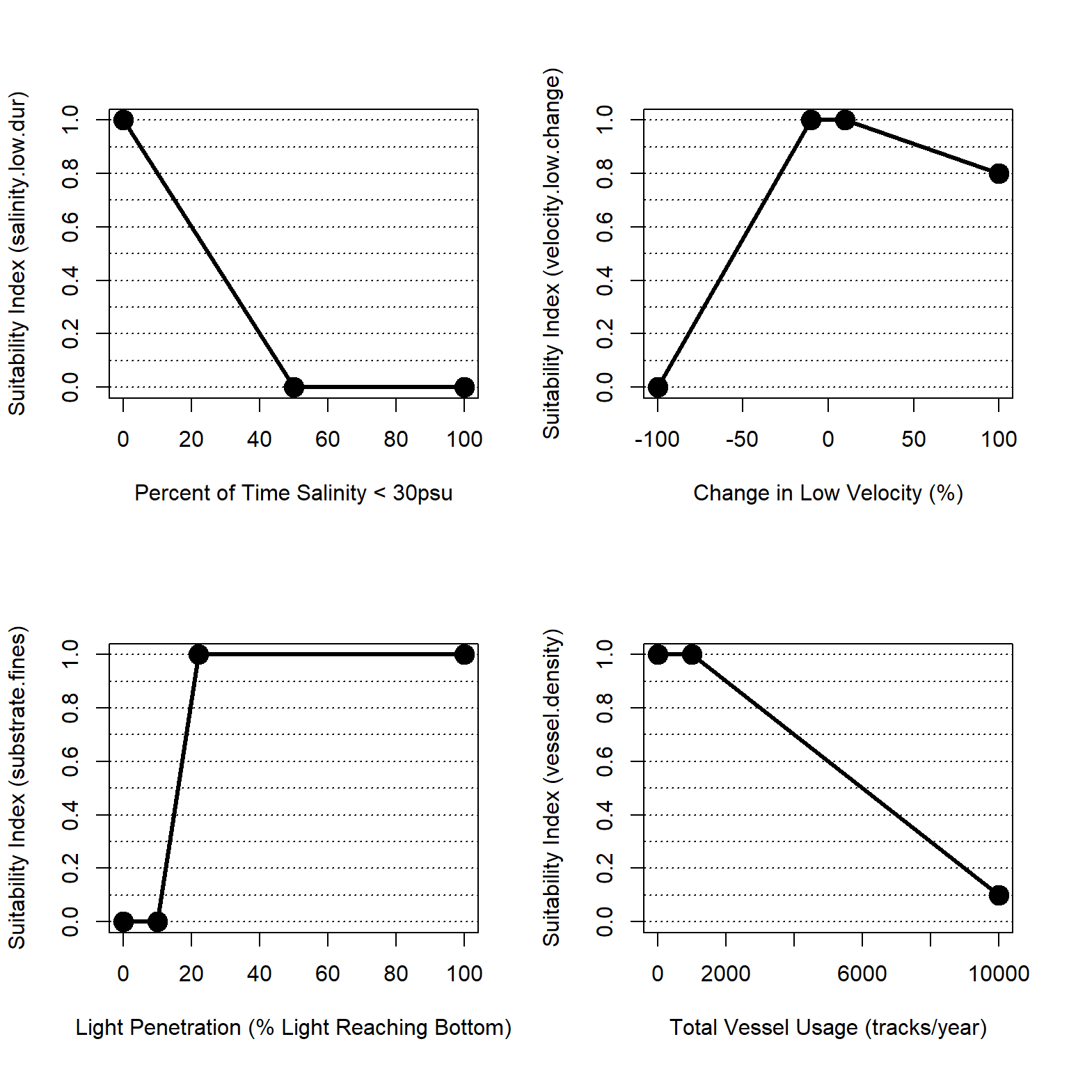
Figure 4.15: Suitability index curves for the marine, deepwater zone.

4.7.1 Salinity

Salinity, often used as a proxy for the total concentration of all dissolved salts in the water, is a key factor in water density that controls the vertical mixing of nutrients and chemicals throughout the water column. Salinity constrains dissolved oxygen concentration and limits speciation of marine zones to euryhaline taxa that are physiological adapted to tolerate hypoosmotic processes (are able to maintain a lower internal ionic concentration than seawater).

For NYBEM, the salinity regime is summarized through a metric of the percent of time salinity is less than the marine ecosystem threshold of 30 psu. This approach assumes that freshwater inputs serve as disturbances on the ecosystem, and higher marine levels of salinity are preferred. Depth-averaged salinity is computed or measured at small time steps over an annual or inter-annual timeframe. These data may then be summarized as an “exceedence curve” with thresholds from 0-100% in 10% intervals. For NYBEM, this exceedence curve is used to calculate the percent of time salinity is less than or equal to 30 psu. This duration metric is then translated into a suitability metric as follows:

\[salinity.low.dur = \begin{pmatrix} -0.02*sal_{dur}+1 & sal_{dur}=0-50\\ 0.0 & sal_{dur}=50-100 \end{pmatrix}\]

Where \(salinity.low.dur\) is a suitability index relative to low salinity periods and \(sal_{dur}\) is the percent of time salinity is less than the threshold for marine habitat (i.e., salinity < 30 psu).

4.7.2 Current Velocity

The marine deepwater environment is subjected to velocity effects from ocean currents and tides that affect vertical and horizontal mixing and flushing of the system, suspended sediment and solids, substrate settlement of taxa, as well as the operation of small and recreational vessels. Low flow conditions allow for the settlement of sediment, possibly burying viable habitat, reducing mixing and flushing, and potentially facilitating hypoxic conditions. Conversely, high velocities scour the benthic environment, prohibiting settling in the substrate by benthic taxa.

Low flow conditions are particularly of concern for these processes, so a representative low velocity (i.e., 10% exceedance probability) is used within NYBEM as a key indicator metric. Suitability is then calculated based on the change in this low velocity relative to a baseline condition. For NYBEM, the baseline condition is assessed as the existing condition for a representative tidal year. Suitability declines linearly beyond a 10% change in this metric from the baseline with sharper decreases as velocities slow.

\[velocity.low.change = \begin{pmatrix} 0.011*vel_{rel}+1.11 & vel_{rel}=-100-10\\ 1.0 & vel_{rel}=-10-10\\ -0.0022*vel_{rel}+1.02 & vel_{rel}>10 \end{pmatrix}\]

Where \(velocity.low.change\) is a suitability index relative to change in low velocity and mixing and \(vel_{rel}\) is the relative change in low velocity from a baseline condition assessed as:

\(vel_{rel}=\frac{vel_{10,f}-vel_{10,b}}{vel_{10,b}}\).

Where \(vel_{10,f}\) is the 10% exceedence velocity for a focal condition and \(vel_{10,b}\) is a 10% exceedence velocity for a baseline condition.

4.7.3 Light

The depth that light reaches within the water column acts as a proxy for the viability of water column turbidity, nutrient loading, and chlorophyll-a production (an essential building block for ocean productivity). As light controls chlorophyll-a production, it may be seen as a limiting factor for algal and particulate organic matter densities, and ultimately the development of harmful algal blooms. Therefore, light provides a meaningful metric for a variety of biological processes in this ecosystem. For the marine deepwater submodel, light availability and suitability are modeled following the same algorithms described for the estuarine subtidal model (See Section 4.4.2.1), which can be summarized in suitability terms as as:

\[light = \begin{pmatrix} 0.0 & PLA<10\\ 0.0833*PLA-0.83 & PLA>70\\ 1.0 & PLA>22\\ \end{pmatrix}\]

Where \(light\) is a suitability index relative to light penetration and \(PLA\) is percent light available (PLA).

4.7.4 Vessel Traffic

Vessel traffic density provides an index for development pressures, both commercial and recreational fishing pressure, and commercial and recreational vessel density pressures on the marine mammal populations within the area (population stress from ship strikes and noise pollution). We quantify these disturbances through a proxy of vessel traffic per year. These data also indicate frequently visited fishing locations and offshore structures. Vessel traffic is obtained from the Automatic Identification System (AIS) database. Lower traffic (less than 1,000 tracks per year) is considered optimal and the suitability decreases with increasing vessel traffic. Suitability scores for are quantified as follows:

\[vessel.density = \begin{pmatrix} 1.0 & ves_{AIS}=0-1000\\ -0.0001*ves_{AIS}+1.1 & ves_{AIS}=1000-10000\\ 0.1 & ves_{AIS}>10000 \end{pmatrix}\]

Where \(vessel.density\) is a suitability index relative to ship traffic and \(ves_{AIS}\) is the annual vessel tracks over a patch from the Automated Information System.

4.7.5 Potential extension of marine, deepwater model

The marine deepwater zone is affected by many processes not included in NYBEM. Future model development could explore the following:

• Dissolved oxygen concentration, a key element for the survival of marine species, limits speciation of marine zones through hypoxia, where low oxygen levels may cause die-offs in marine species. Dissolved oxygen concentrations act as a proxy for pelagic, demersal and benthic fauna biomass (abundance/diversity of phytoplankton, zooplankton, fish, marine turtles, birds and mammals). Data could potentially be integrated from sources such as permanent monitoring stations, as supported by NYC DEP Monitoring Stations (McFarland and Hare 2018), Jamaica Bay Eutrophication Model (Fischbach et al. 2018), frameworks such as the Chesapeake Bay model (Cerco and Cole 1993), and the EPA Long Island Sound integrated model (underway).
  
• Water temperature acts as a control for the majority of the chemical (dissolved nutrients, pH, density, and photosynthesis), biological (respiration and metabolic rates, taxa development, and migrations) and physical (ice formation and thermal stratification of the water column) properties of a marine ecosystem. Methods could be adapted from the Winter flounder habitat suitability model (Banner and Schaller 2001), VIMS 2018 habitat suitability models, or the USACE Harbor monitoring (USACE 2013), and data could potentially be extracted from MARACOOS Monthly Sea Surface Temperature via the MARCO Mid-Atlantic Ocean Data Portal or via hydrodynamic model outputs.
  
• The wave environment affects many variables with the New York Bight: vertical and horizontal mixing and flushing of the physical and chemical properties of the water, suspended sediment and solids, substrate settlement of taxa, and commercial and recreational vessel traffic. Wave height and wave refraction could be assessed from analytical software such as STWAVE (Byrnes et al. 2004).
  
• In the present iteration of NYBEM, light attenuation is assumed to be dependent on a single light coefficient (\(K_{d}\)). However, light attentuation can vary significantly based on suspended sediment concentration, algal processes, or water color, all of which may vary in time. Future version of the model could also consider spatially distributed data sets of light coefficients such as those by NOAA.

4.8 nybem R-package

Rapid timelines and iterative development encourage a transparent approach for model development and documentation. We adopt a growing family of methods for “reproducible research,” which embrace transparent coding techniques and data sharing. Specifically, R Markdown is applied to develop and document models, which are coded in the R Statistical Software. Similarly, all model code is contained within a transportable R-package (i.e., nybem) following common development procedures.

All model code for the nybem R-package is available via github. Generally speaking, a package can be thought of as a fundamental unit of code that can include functions, data, documentation, and tests (Wickham and Bryan 2019). Packages then provide a transportable and reproducible mechanism for code sharing and publication. The nybem package contains two sets of functions and one data object storing suitability curves (Figure 4.1). The first set of functions can largely be thought of as habitat mapping functions, which delineate NYBEM habitat zones. The second set of functions compute habitat quality using a general set of algorithms and data management functions. The data object contains suitability curve data as described in Sections 4.2-4.7. These topics will be treated separately in 4.8.1-4.8.3, respectively. Model code may be inspected on the nybem github repo, and in-line documentation further describes the logic of the model.

Notably, all functions and data presented in nybem are modular and can be used independently. For instance, ecosystems could be delineated from empirical data (e.g., field or tide gauge data) or modeled hydrodynamic data. Similarly, habitat quality assessments could be conducted for one of the six habitat types without consideration of the others.

4.8.1 Habitat Mapping Functions

The first set of functions in nybem collectively allow for delineation and mapping of the six major ecosystem types described in Sections 3.2. Three functions execute the logic of habitat delineation shown in Section 4.1.

set_tidal_zone delineates four types of tidal regimes: deepwater, subtidal, intertidal, and upland (coded as outputs of 1, 2, 3, and 4, respectively). Inputs to this function are bed elevation, mean lower low water (MLLW), and mean higher high water (MHHW). Here is the relevant portion of the function:

set_tidal_zone <- function(bedelev, MLLW, MHHW){
  # ...
  # Assign tidal zone values
  tidal_zone <- nybem::ifelse(bed_elevation <= -2,   1,          # Deep
                nybem::ifelse(bed_elevation <= MLLW, 2,          # Subtidal
                nybem::ifelse(bed_elevation <= MHHW, 3,          # Intertidal
                nybem::ifelse(bed_elevation >  MHHW, 4, 0))))    # Upland
  ## ...
  return(tidal_zone)
}

set_salinity_zone delineates three salinity regimes: marine, estuarine, and freshwater (coded as outputs of 1, 2, and 3, respectively). Inputs to this function are a representative low salinity. Here is the relevant portion of the function:

set_salinity_zone <- function(salinity){
  # ...
  #Assign salinity zone
  salinity_zone <- ifelse(salinity >= estuarine_marine_break, 1,     # Marine
                   ifelse(salinity <  estuarine_marine_break &
                          salinity >= fresh_estuarine_break, 2,      # Estuarine
                   ifelse(salinity <  fresh_estuarine_break, 3, 0))) # Fresh
  # ...
  return(salinity_zone)
}

set_habitat_zone combines tidal and salinity zonation into seven major ecosystem types: upland, marine deepwater, marine subtidal, marine intertidal, estuarine subtidal, estuarine intertidal, and freshwater tidal (coded as 1, 2, 3, 4, 5, 6, and 7, respectively). Notably, upland ecosystems are outside of the model domain and do not include habitat suitability models below. Here is the relevant portion of the function:

set_habitat_zone <- function(tidal_zone, salinity_zone){
  # ...
  #Assign habitat zone
  habitat_zone <- ifelse(tidal_zone == 4, 1,
                  ifelse(salinity_zone == 1 &  tidal_zone == 1,  2,
                  ifelse(salinity_zone == 1 &  tidal_zone == 2,  3,
                  ifelse(salinity_zone == 1 &  tidal_zone == 3,  4,
                  ifelse(salinity_zone == 2 & (tidal_zone == 1 |
                                               tidal_zone == 2), 5,
                  ifelse(salinity_zone == 2 &  tidal_zone == 3,  6,
                  ifelse(salinity_zone == 3 & (tidal_zone == 1 |
                                               tidal_zone == 2 |
                                               tidal_zone == 3), 7, 0)))))))
  # ...
  return(habitat_zone)
}

4.8.2 Habitat Quality Functions

This group of functions computes habitat quality and can be thought of as the major computational engine of nybem. Two functions in particular conduct the bulk of habitat suitability calculations. SIcalc computes suitability for a given set of suitability curves (Section 4.8.3) and a set of user-defined inputs. HSIcalc computes an overarching habitat suitability index from multiple suitability indices (i.e., the output of SIcalc). These functions are adapted from an existing R-package for single patch habitat suitability analyses, ecorest (McKay and Hernandez-Abrams 2020). The prior model did not contain raster functionality for spatially explicit mapping, and the functions were adapted to handle this different data format.

SIcalc computes habitat suitability relative to multiple variables and user-defined inputs. For instance, NYBEM’s freshwater tidal submodel include suitability curves associated with salinity, vegetation cover, and episodic flooding and sediment deposition (Section 4.2). SIcalc takes in the breakpoints of these suitability curves along with user-defined inputs for a given site and scenario. Suitability index curves may be specified as either categorical or continuous variables. For categorical variables, the model uses a look-up approach to identify suitability associated with that class. For continuous variables, the model computes suitability by linearly interpolating suitability values associated with the user inputs. Additional detail may be found in the ecorest reference manual.

SIcalc <- function (SI, input_proj) {
  # Set number of metrics in the SI model (count of breakpoint-SI pairs)
  nSI <- length(colnames(SI))/2
  # input_proj parameter must be list to preserve metric data type
  if(!is.list(input_proj)) {stop("input_proj must be a list")}
  # Number of inputs must match number of model metrics
  if(length(input_proj) != nSI) {
    stop("Number of inputs does not equal required SI model metrics")}

  # Iterate through each pair of model metric and inputs
  SI_out <- list()
  for(i in 1:nSI) {
    # Set current model values
    current_metric_column <- 2 * i - 1
    current_si_column     <- 2 * i
    metric_vector <- SI[, current_metric_column]
    si_vector     <- SI[, current_si_column]
    current_metric_continuous <- is.numeric(metric_vector)

    # Set current input_proj values
    current_input_raster <- nybem::is_RasterLayer(input_proj[[i]])
    if(current_input_raster) {
      current_input <- raster::getValues(input_proj[[i]])
    } else {
      current_input <- input_proj[[i]]
    }

    # Check if current metric and input are of the same data type
    current_input_continuous <- all(
                    is.numeric(current_input),
                    if(current_input_raster) {!input_proj[[i]]@data@isfactor})
    if(current_input_continuous != current_metric_continuous) {
      stop("Input data types must match data types of SI model metrics")}

    # Calculate continuous SI
    if(current_metric_continuous == TRUE) {
      si <- approx(metric_vector, si_vector,
                   xout = current_input,
                   method = "linear", rule = 2, ties = "ordered")$y
    }

    # Calculate categorical SI
    if(current_metric_continuous != TRUE) {
      # Create named vector for lookup
      get_cat_metric <- si_vector
      names(get_cat_metric) <- metric_vector

      # Get si values for current_input
      si <- unname(get_cat_metric[current_input])
    }

    # Assign si to SI_out[[i]]
    if(current_input_raster) {
      SI_out[[i]] <- raster::setValues(input_proj[[i]], si)
    } else {
      SI_out[[i]] <- si
    }
  }
  return(SI_out)
}

HSIcalc takes in suitability indices associated with multiple variables and computes and overarching habitat suitability index, which can be thought of as a metric of ecosystem condition or integrity. The model computes suitability based on an arithmetic mean although other forms of combination (e.g., geometric mean, minimums) could be incorporated into future versions.

HSIcalc <- function(si_list, method = "mean") {
  # si_list parameter must be list to preserve metric data type
  if(!is.list(si_list)) {stop("si_list must be a list")}
  if(!(method %in% c("mean"))) {
    stop("method must be one of 'mean', ")}

  # Check input for rasters
  raster_input <- any(unlist(lapply(si_list, is_RasterLayer)))

  # Create a raster brick
  if(raster_input) {
    si <- raster::brick(si_list)
  }

  # Convert list to vector for non-rasters
  if(!raster_input) {
    si <- unlist(si_list)
  }

  if(method == "mean") {
    if(!raster_input) {
      hsi_score <- mean(si, na.rm = TRUE)
    }

    if(raster_input) {
      hsi_score <- raster::calc(si, mean)
    }
  }

  return(hsi_score)
}

A variety of small scale utility functions were also needed to manage input / output data and support these functions. The underlying code for these functions can be found in the nybem package and help documentation, but it is not presented here in the interest of brevity. In general, the utility functions have the following goals.

• is_RasterLayer verifies that the input to a given function is of class raster::RasterLayer.
  
• is_cat_raster verifies that the input to a given function is of class raster::RasterLayer and is a factor.
  
• ifelse provides capacity to execute if-else logic statements on raster data.
  
• write_cat_tiff writes a categorical raster that preserves color schemes in the raster attribute table for ESRI reverse compatibility.
  
• write_cont_tiff writes a continuous raster that preserves color schemes in the raster attribute table for ESRI reverse compatibility.
  
• raster_fig creates a raster figure cropped to the specified extent.
  
• na_outside_model sets all HSI values outside of the modeled habitat zone to -1 to distinguish areas inside the study area, but outside the modeled habitat zone.
  
• name_model assigns a name to a raster HSI model. Used for processing individual models into alternatives analysis for a study area.
  
• model_summary displays a brief set of result summaries for each HSI model.
  
• summarize_by_poly summarizes the raster HSI model by polygon.
  
• are_colors determines if the input is a vector of valid colors according to the grDevices::col2rgb function.
  
• has_colortable determines if a RasterLayer has a valid colortable defined.

4.8.3 Habitat Suitability Curves

The final major component of the nybem package is a single data object that stores all of the habitat suitability curves. This object is a list format with each list element holding the set of suitability curves associated with one submodel (e.g., freshwater tidal). The following code displays this list for comparison against suitability curves presented in Sections 4.2-4.7.

#Store models in a single list
nybem.submodels <- list(NYBEM.fresh.tid, NYBEM.est.int, 
                        NYBEM.est.sub.hard, NYBEM.est.sub.soft.sav, NYBEM.est.sub.soft.clam,
                        NYBEM.mar.int, NYBEM.mar.sub, NYBEM.mar.deep)
names(nybem.submodels) <- c("fre.tid", "est.int", 
                            "est.sub.hard", "est.sub.soft.sav", "est.sub.soft.clam", 
                            "mar.int", "mar.sub", "mar.deep")

#Show model data
nybem.submodels

## $fre.tid
##   salinity.per salinity.SIV veg.cover.per veg.cover.SIV deposition
## 1            0            1             0           0.1          1
## 2           20            0            57           0.5          2
## 3          100            0           100           1.0          5
## 4           NA           NA            NA            NA         NA
##   deposition.SIV
## 1              0
## 2              1
## 3              1
## 4             NA
## 
## $est.int
##   erosion erosion.SIV veg.cover.per veg.cover.SIV deposition deposition.SIV
## 1     -50           1             0           0.1          0              1
## 2      10           1           100           1.0          1              0
## 3      50           0            NA            NA         NA             NA
##   land.use.per land.use.SIV shoreline.m shoreline.SIV
## 1            0            1           0           0.5
## 2           10            1         100           1.0
## 3          100            0         500           1.0
## 
## $est.sub.hard
##   cultch cultch.SIV MAS MAS.SIV AS AS.SIV
## 1      0          0   0    0.00  0   0.00
## 2    100          1   2    0.00  5   0.00
## 3     NA         NA   4    0.05 10   1.00
## 4     NA         NA   6    0.50 15   1.00
## 5     NA         NA   8    1.00 20   0.60
## 6     NA         NA  40    1.00 25   0.25
## 7     NA         NA  NA      NA 30   0.10
## 8     NA         NA  NA      NA 40   0.00
## 9     NA         NA  NA      NA NA     NA
## 
## $est.sub.soft.sav
##   substrate.sav substrate.sav.SIV light.PLA light.SIV vessel.density
## 1             0               1.0         0         0              0
## 2            70               1.0        10         0           1000
## 3           100               0.1        22         1          10000
## 4            NA                NA       100         1             NA
##   vessel.density.SIV
## 1                1.0
## 2                1.0
## 3                0.1
## 4                 NA
## 
## $est.sub.soft.clam
##   salinity.clam salinity.clam.SIV substrate.clam.fines substrate.clam.SIV Isav
## 1           0.0              0.00                    0               1.00  0.0
## 2          12.0              0.00                   50               0.75  0.2
## 3          12.5              0.25                   90               0.25  0.8
## 4          20.0              0.75                  100               0.00  1.0
## 5          25.0              1.00                   NA                 NA   NA
## 6          35.0              1.00                   NA                 NA   NA
## 7          45.0              0.00                   NA                 NA   NA
##   Isav.SIV
## 1        1
## 2        1
## 3        0
## 4        0
## 5       NA
## 6       NA
## 7       NA
## 
## $mar.int
##   beach.slope.per beach.slope.SIV trel exp.dur.SIV land.use.per land.use.SIV
## 1               0               1 0.00           0            0            1
## 2              10               1 0.25           1           10            1
## 3              30               0 0.75           1          100            0
## 4              NA              NA 1.00           0           NA           NA
##   shoreline.m shoreline.SIV
## 1           0             0
## 2         100             1
## 3         500             1
## 4          NA            NA
## 
## $mar.sub
##   velocity velocity.SIV substrate.fines substrate.SIV light.PLW light.SIV
## 1        0          0.6               0           1.0         0         0
## 2       25          1.0             100           0.1        10         0
## 3       50          1.0              NA            NA        22         1
## 4      100          0.0              NA            NA       100         1
##   vessel.density vessel.density.SIV
## 1              0                1.0
## 2           1000                1.0
## 3          10000                0.1
## 4             NA                 NA
## 
## $mar.deep
##   salinity.low.dur salinity.low.SIV velocity.low.change velocity.low.SIV
## 1                0                1                -100              0.0
## 2               50                0                 -10              1.0
## 3              100                0                  10              1.0
## 4               NA               NA                 100              0.8
##   light.PLW light.SIV vessel.density vessel.density.SIV
## 1         0         0              0                1.0
## 2        10         0           1000                1.0
## 3        22         1          10000                0.1
## 4       100         1             NA                 NA